3.11 — ℝⁿ-এ Lebesgue Integration¶

এই অধ্যায়ে কী শিখব: $\mathbb{R}^n$-এ Borel ও Lebesgue measure কীভাবে product measure হিসেবে গড়ে ওঠে; $\mathbb{R}^n$-এ integration; unit ball $B_n$-এর volume-এর বিখ্যাত formula Fubini দিয়ে পেতে শিখব; mixed partial derivatives-এর সমতা Fubini থেকে প্রমাণ করব; এবং Part 3-এর সামগ্রিক চিত্র — Riemann-এর কোথায় সমস্যা ছিল, Lebesgue কীভাবে সব ঠিক করল।

উৎস (source): Lebesgue ও Fubini (ℝⁿ-এ integration)।

১. কেন শিখব? (Motivation)¶

Part 3-এর শুরুতে (3.1 — Outer Measure) আমরা বেরিয়েছিলাম একটা প্রশ্নের উত্তর খুঁজতে: Riemann integral-এর সীমাবদ্ধতা দূর করা কীভাবে সম্ভব? পুরো Part 3 জুড়ে পেয়েছি:

Measure theory (3.1–3.5): measurable sets ও Lebesgue measure।
Lebesgue integral (3.7–3.8): DCT, MCT, Fatou।
Differentiation (3.9): Lebesgue Differentiation Theorem।
Product measures (3.10): Tonelli ও Fubini।

এখন শেষ ধাপ: এই সব theory $\mathbb{R}^n$-এ একত্রিত করা। $\mathbb{R}^n$-এর Lebesgue measure হলো product measure — $n$-টা real line-এর Lebesgue measure-এর গুণফল।

এই অধ্যায়ে আমরা দেখব:

Borel subsets of $\mathbb{R}^n$ কীভাবে product structure পায়।
$\lambda_n = \lambda_{n-1} \times \lambda_1$ দিয়ে inductive definition।
Unit ball-এর volume — একটা সুন্দর recursive formula।
Mixed partials-এর equality — Fubini-র একটা elegant application।
পুরো Part 3-এর recap।

২. মূল ধারণা (Core idea)¶

$\mathbb{R}^n$-কে product হিসেবে দেখা¶

$\mathbb{R}^n = \mathbb{R}^{n-1} \times \mathbb{R}$। এই decomposition বারবার করা যায়:

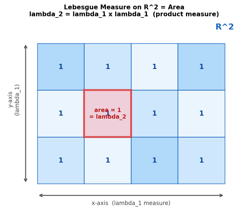\[\mathbb{R}^n = \underbrace{\mathbb{R} \times \mathbb{R} \times \cdots \times \mathbb{R}}_{n\text{ কপি}}.\]

চিত্র: ℝ²-এ Lebesgue measure = area: unit squares-এর grid। lambda_2 = lambda_1 x lambda_1 (product measure)।

তাই স্বাভাবিক: $\lambda_n = \lambda_1 \times \lambda_1 \times \cdots \times \lambda_1$ ($n$-বার)। একটু সাবধানে inductively define করলে এটাই Lebesgue measure on $\mathbb{R}^n$।

Unit ball volume-এর স্বজ্ঞা¶

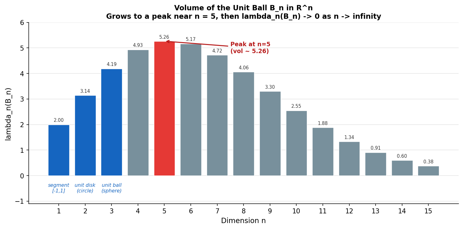
$B_n = \{x \in \mathbb{R}^n : \|x\| < 1\}$। নিচের চিত্রে দেখা যাচ্ছে volume-এর pattern:

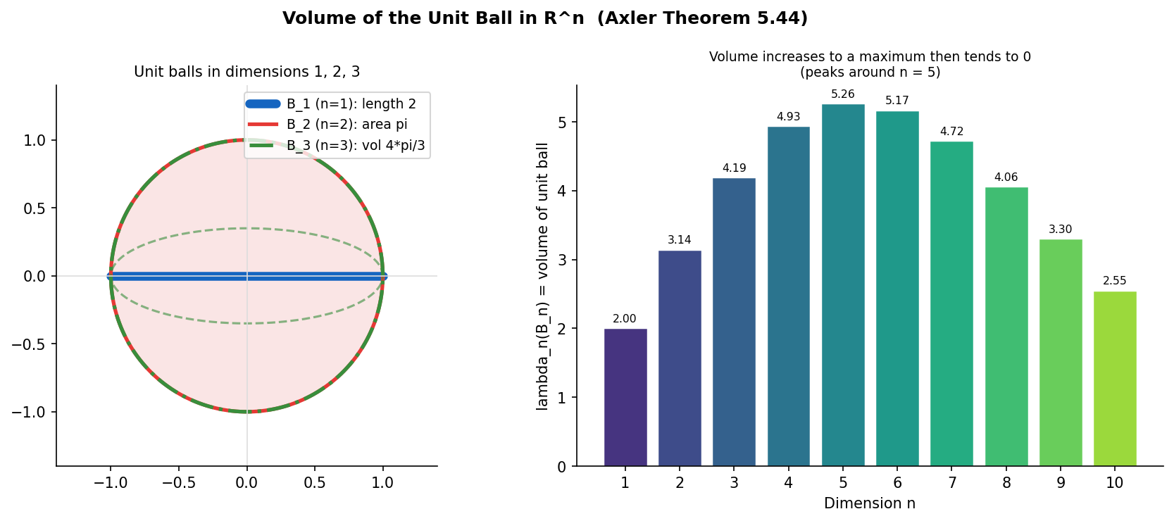Unit ball volume in R^n চিত্র ১: বাঁয়ে: $B_1$ (রেখাখণ্ড), $B_2$ (বৃত্ত), $B_3$ (গোলক)। ডানে: $\lambda_n(B_n)$ বনাম $n$। volume $n=5$ পর্যন্ত বাড়ে, তারপর $0$-এর দিকে যায়।

আশ্চর্যের বিষয়: $n \to \infty$-তে unit ball-এর volume $\to 0$! একটা $n$-মাত্রিক unit ball তার circumscribed cube $[-1,1]^n$ (volume $= 2^n$)-এর ক্রমশ ছোট অংশ হয়ে যায়।

৩. সংজ্ঞা ও উপপাদ্য (Definitions & Theorems)¶

Borel Sets in $\mathbb{R}^n$¶

সংজ্ঞা

$\mathbb{R}^n$-এর Borel subset হলো $\mathbb{R}^n$-এর সব open sets ধারণ করা সবচেয়ে ছোট σ-algebra $\mathcal{B}^n$-এর elements।

মূল ফলাফল:

\[\mathcal{B}^m \otimes \mathcal{B}^n = \mathcal{B}^{m+n}.\]

মানে: $\mathbb{R}^m$ ও $\mathbb{R}^n$-এর Borel sets-এর product σ-algebra = $\mathbb{R}^{m+n}$-এর Borel σ-algebra।

Proof sketch: Open cubes in $\mathbb{R}^{m+n}$ = products of open cubes in $\mathbb{R}^m$ ও $\mathbb{R}^n$। Open cubes generate $\mathcal{B}^{m+n}$। তাই $\mathcal{B}^{m+n} \subseteq \mathcal{B}^m \otimes \mathcal{B}^n$। উল্টোটাও একইভাবে। $\square$

Lebesgue Measure on $\mathbb{R}^n$¶

সংজ্ঞা

$\mathbb{R}^n$-এ Lebesgue measure $\lambda_n$ inductively define হয়:

$\lambda_n = \lambda_{n-1} \times \lambda_1,$

যেখানে $\lambda_1$ হলো $(\mathbb{R}, \mathcal{B}^1)$-এর Lebesgue measure। Base case: $\lambda_1$ = standard।

$\mathcal{B}^n = \mathcal{B}^{n-1} \otimes \mathcal{B}^1$ (উপরের ফলাফল থেকে), তাই $\lambda_n$ সত্যিই $\mathcal{B}^n$-এ defined।

Integration on $\mathbb{R}^n$: Tonelli ব্যবহার করে, যেকোনো $E \in \mathcal{B}^n$-এর জন্য:

\[\lambda_n(E) = \int_{\mathbb{R}^{n-1}}\int_\mathbb{R} \chi_E(x,y)\,d\lambda_1(y)\,d\lambda_{n-1}(x).\]

Tonelli-কে বারবার apply করে $\lambda_n(E)$-কে $n$-টা one-dimensional integral-এর iterated form-এ লেখা যায়।

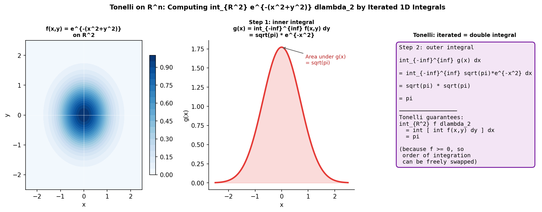$Tonelli on ℝ²: e^{-(x²+y²)} integral ste$ চিত্র: Tonelli on ℝ²: e^{-(x²+y²)} integral step-by-step — double integral = iterated 1D integrals = π।

Translation invariance: $\lambda_n(a + E) = \lambda_n(E)$ সব $a \in \mathbb{R}^n$-এর জন্য — Lebesgue measure translation-invariant।

Dilation: $\lambda_n(tE) = t^n \lambda_n(E)$ for $t > 0$ — natural scaling।

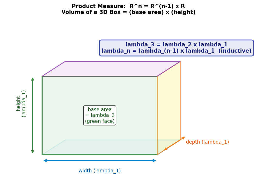চিত্র: ℝⁿ-এ measure product হিসেবে: 3D box-এর volume = base area × height। lambda_n = lambda_(n-1) × lambda_1।

Volume of the Unit Ball — Worked Computation¶

এটা।

Theorem: Volume of Unit Ball in $\mathbb{R}^n$

\[\lambda_n(B_n) = \begin{cases} \dfrac{\pi^{n/2}}{(n/2)!} & \text{যদি }n\text{ জোড়}, \\[8pt] \dfrac{2^{(n+1)/2}\pi^{(n-1)/2}}{1\cdot 3 \cdot 5 \cdots n} & \text{যদি }n\text{ বিজোড়}. \end{cases}\]

প্রথম কয়েকটা মান:

$n$	$\lambda_n(B_n)$	আনুমানিক
1	$2$	2.00
2	$\pi$	3.14
3	$4\pi/3$	4.19
4	$\pi^2/2$	4.93
5	$8\pi^2/15$	5.26
6	$\pi^3/6$	5.17
10	$\pi^5/120$	2.55

Recursive formula (মূল idea): $\mathbb{R}^n = \mathbb{R}^2 \times \mathbb{R}^{n-2}$ লিখলে:

\[\lambda_n(B_n) = \int_{\mathbb{R}^2}\int_{\mathbb{R}^{n-2}} \chi_{B_n}(x,y)\,dy\,dx.\]

Fixed $x = (x_1, x_2) \in \mathbb{R}^2$: $\chi_{B_n}(x,y) = 1 \iff \|y\| < (1 - \|x\|^2)^{1/2}$ (যখন $\|x\| < 1$)।

তাই ভেতরের integral = $\lambda_{n-2}\!\left((1-\|x\|^2)^{1/2} B_{n-2}\right) = (1-\|x\|^2)^{(n-2)/2}\lambda_{n-2}(B_{n-2})$ (dilation formula)।

তাই:

\[\lambda_n(B_n) = \lambda_{n-2}(B_{n-2})\int_{B_2}(1-x_1^2-x_2^2)^{(n-2)/2}\,d\lambda_2.\]

Polar coordinates ($d\lambda_2 = r\,dr\,d\theta$):

\[= \lambda_{n-2}(B_{n-2})\int_{-\pi}^{\pi}\int_0^1(1-r^2)^{(n-2)/2}r\,dr\,d\theta = \lambda_{n-2}(B_{n-2})\cdot 2\pi\cdot\frac{1}{n} = \frac{2\pi}{n}\lambda_{n-2}(B_{n-2}).\]

Recursive formula: $\lambda_n(B_n) = \dfrac{2\pi}{n}\lambda_{n-2}(B_{n-2})$, base cases $\lambda_1(B_1) = 2$, $\lambda_2(B_2) = \pi$।

Closed form থেকে: $\lim_{n\to\infty}\lambda_n(B_n) = 0$। (Exercise 12 in।)

চিত্র: Unit ball-এর volume বনাম dimension n: n=5 পর্যন্ত বাড়ে, তারপর 0-তে যায়।

Equality of Mixed Partial Derivatives via Fubini¶

Elementary calculus থেকে মনে আছে: বেশিরভাগ ক্ষেত্রে $\partial_x\partial_y f = \partial_y\partial_x f$। Fubini এটার একটা clean proof দেয়:

Theorem: Mixed Partial Derivatives

$G \subseteq \mathbb{R}^2$ open, $f: G \to \mathbb{R}$। ধরো $D_1 f$, $D_2 f$, $D_1(D_2 f)$, $D_2(D_1 f)$ সবই exist ও continuous। তাহলে:

$D_1(D_2 f) = D_2(D_1 f) \quad \text{on } G.$

Proof (Fubini-ভিত্তিক): Fix $(a,b) \in G$। Small square $S_\delta = [a, a+\delta]\times[b, b+\delta] \subseteq G$ নাও।

Fubini দিয়ে:

\[\int_{S_\delta} D_1(D_2 f)\,d\lambda_2 = \int_b^{b+\delta}\int_a^{a+\delta} D_1(D_2 f)(x,y)\,dx\,dy\]

\[= \int_b^{b+\delta}\big[(D_2 f)(a+\delta, y) - (D_2 f)(a,y)\big]\,dy \quad \text{(FTC)}\]

\[= f(a+\delta, b+\delta) - f(a+\delta, b) - f(a, b+\delta) + f(a,b). \quad \text{(FTC আবার)}\]

একইভাবে $\int_{S_\delta} D_2(D_1 f)\,d\lambda_2$-ও একই মান দেয়। তাই:

\[\int_{S_\delta}[D_1(D_2 f) - D_2(D_1 f)]\,d\lambda_2 = 0 \quad \text{সব ছোট } \delta\text{-এর জন্য}.\]

$D_1(D_2 f) - D_2(D_1 f)$ continuous এবং সব ছোট rectangle-এ integral 0 → $D_1(D_2 f) = D_2(D_1 f)$ everywhere। $\square$

৪. উদাহরণ ও Analogy¶

Example 1: $\lambda_2$ of a Rectangle¶

$[a_1, b_1] \times [a_2, b_2]$-এর Lebesgue measure:

\[\lambda_2([a_1,b_1]\times[a_2,b_2]) = (\lambda_1\times\lambda_1)([a_1,b_1]\times[a_2,b_2]) = (b_1-a_1)(b_2-a_2) = \text{area}.\]

সঠিক! Product measure আয়তক্ষেত্রের ক্ষেত্রফল = দৈর্ঘ্য × প্রস্থ দেয়।

Example 2: Unit Ball Volume Verification for $n=3$¶

Recursive formula: $\lambda_3(B_3) = \frac{2\pi}{3}\lambda_1(B_1) = \frac{2\pi}{3}\cdot 2 = \frac{4\pi}{3}$। ✓ (elementary formula-র সাথে মেলে!)

Example 3: Integration on $\mathbb{R}^3$¶

$f(x,y,z) = e^{-(x^2+y^2+z^2)}$ on $\mathbb{R}^3$। Tonelli-কে তিনবার apply করলে:

\[\int_{\mathbb{R}^3} f\,d\lambda_3 = \left(\int_\mathbb{R} e^{-x^2}\,dx\right)^3 = (\sqrt{\pi})^3 = \pi^{3/2}.\]

(কারণ integrand $= g(x)g(y)g(z)$, তাই integral factorizes।)

Analogy: Volume by Slicing¶

$\mathbb{R}^3$-এ একটা region-এর volume মাপতে horizontal slices নাও। প্রতিটা slice-এর area হিসেব করো, সব slices যোগ করো — এটাই Fubini-র idea। এবং আমরা যেকোনো direction-এ slice করতে পারি (Tonelli guarantee দেয়)।

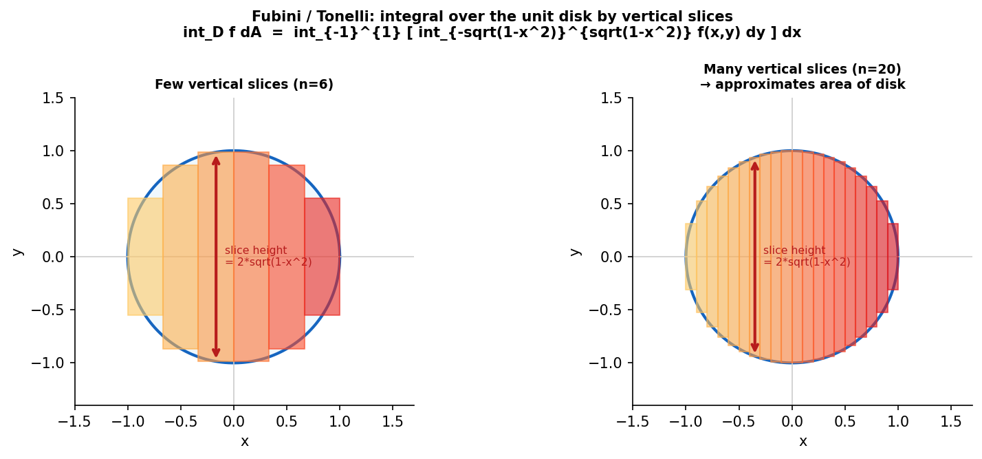চিত্র: Fubini দিয়ে unit disk-এ integration: vertical slices নিয়ে 2D integral-কে iterated 1D integral-এ রূপান্তর।

৫. সাধারণ ভুল (Common mistakes)¶

$\mathcal{B}^m \otimes \mathcal{B}^n = \mathcal{B}^{m+n}$ না জানা। এটা trivial নয় — explicitly prove করতে হয়। এছাড়া $\lambda_{m+n} = \lambda_m \times \lambda_n$ বলার ভিত্তি নেই।
Dilation formula ভুল করা। $\lambda_n(tE) = t^n\lambda_n(E)$ — factor $t^n$, $t$ নয়। কারণ $n$-মাত্রায় linear scaling $n$-ঘাতে volume বাড়ায়।
Unit ball volume-কে monotone ভাবা। $\lambda_n(B_n)$ প্রথমে বাড়ে, তারপর কমে শূন্যে যায়। $n=5$-এ সর্বোচ্চ।
Mixed partials সবসময় equal ভাবা। continuity ছাড়া হয় না। : $f(x,y) = xy(x^2-y^2)/(x^2+y^2)$ ($(0,0)$-তে $0$) একটা counterexample।
$\mathbb{R}^n$-এ integral-কে "just multiply" ভাবা। $\int_{\mathbb{R}^n} f\,d\lambda_n \neq \prod_{i=1}^n \int_\mathbb{R} f_i\,d\lambda_1$ সাধারণ $f$-এর জন্য। এটা শুধু কাজ করে যখন $f(x_1,\ldots,x_n) = f_1(x_1)\cdots f_n(x_n)$ (separable form)।

৬. এক্সারসাইজ (Exercises)¶

Recursive formula $\lambda_n(B_n) = \frac{2\pi}{n}\lambda_{n-2}(B_{n-2})$ ব্যবহার করে $\lambda_4(B_4)$ ও $\lambda_5(B_5)$ বের করো। উপরের table-এর সাথে মিলিয়ে নাও।
$\lambda_3$-এ unit sphere $S^2 = \{x\in\mathbb{R}^3: \|x\|=1\}$-এর measure কত? কেন?
Fubini ব্যবহার করে $\int_{\mathbb{R}^2} e^{-(x^2+y^2)}\,d\lambda_2$ বের করো। এটা কি $(\int_\mathbb{R} e^{-x^2}\,dx)^2$-এর সমান? কেন?
$f(x,y) = x^2 + y^2$ on the disk $D = \{(x,y): x^2+y^2 \leq 1\}$। Fubini দিয়ে $\iint_D f\,dA$ বের করো (polar coordinates নয়, সরাসরি)।
দেখাও যে $\mathbb{R}^n$-এ Lebesgue measure translation-invariant: $\lambda_n(a+E) = \lambda_n(E)$ সব $a\in\mathbb{R}^n$, $E\in\mathcal{B}^n$-এর জন্য।
Mixed partials theorem apply করো $f(x,y) = x^3y^2 - 2xy^3$-এর জন্য। $D_1(D_2 f) = D_2(D_1 f)$ সরাসরি compute করে verify করো।
$\lim_{n\to\infty}\lambda_n(B_n) = 0$ প্রমাণ করো (hint: Stirling's approximation বা recursive formula ব্যবহার করো)।
$f: \mathbb{R}^2 \to \mathbb{R}$, $f(x,y) = \mathbf{1}_{[0,1]^2}(x,y) \cdot (x-y)$। $\int_{\mathbb{R}^2} f\,d\lambda_2$ বের করো। এর জন্য Fubini কি প্রযোজ্য?

৭. সমাধান (ব্যাখ্যাসহ)¶

১-নং সমাধান দেখাও

Recursive formula: $\lambda_n(B_n) = \frac{2\pi}{n}\lambda_{n-2}(B_{n-2})$।

$\lambda_4(B_4) = \frac{2\pi}{4}\lambda_2(B_2) = \frac{\pi}{2}\cdot\pi = \frac{\pi^2}{2} \approx 4.93$। ✓

$\lambda_5(B_5) = \frac{2\pi}{5}\lambda_3(B_3) = \frac{2\pi}{5}\cdot\frac{4\pi}{3} = \frac{8\pi^2}{15} \approx 5.26$। ✓

২-নং সমাধান দেখাও

$S^2 = \partial B_3$ হলো একটা 2-dimensional surface $\mathbb{R}^3$-এ।

$\lambda_3(S^2) = \lambda_3(\partial B_3) = 0$ কারণ sphere = $B_3$ আর $\bar{B}_3$-এর পার্থক্য = $\{x: \|x\| = 1\}$।

$\lambda_3$-measure measure করে 3D volume। $S^2$ হলো একটা 2D surface, যার 3D "thickness"= 0। তাই $\lambda_3(S^2) = 0$।

(এটা যেকোনো $k$-dimensional manifold $k < n$-এর জন্য $\lambda_n$-measure = 0।)

৩-নং সমাধান দেখাও

$f(x,y) = e^{-(x^2+y^2)} = e^{-x^2}\cdot e^{-y^2}$ — separable।

Tonelli (nonneg):

$\int_{\mathbb{R}^2} e^{-(x^2+y^2)}\,d\lambda_2 = \int_\mathbb{R}\int_\mathbb{R} e^{-x^2}e^{-y^2}\,dy\,dx = \int_\mathbb{R} e^{-x^2}\left(\int_\mathbb{R} e^{-y^2}\,dy\right)dx.$

$\int_\mathbb{R} e^{-y^2}\,dy = \sqrt{\pi}$ (Gaussian integral — এটা polar coordinates দিয়ে যায়, বা পরিচিত result হিসেবে ধরি)।

তাই $\int_{\mathbb{R}^2} e^{-(x^2+y^2)}\,d\lambda_2 = \sqrt{\pi}\cdot\int_\mathbb{R} e^{-x^2}\,dx = \sqrt{\pi}\cdot\sqrt{\pi} = \pi$।

হ্যাঁ, এটা $(\int_\mathbb{R} e^{-x^2}\,dx)^2 = (\sqrt{\pi})^2 = \pi$ — সমান। ✓ Separable function-এর জন্য এটাই হয়।

৪-নং সমাধান দেখাও

$D = \{(x,y): x^2+y^2\leq 1\}$। Fubini (fix $x$, integrate $y$):

$\iint_D (x^2+y^2)\,dA = \int_{-1}^1\int_{-\sqrt{1-x^2}}^{\sqrt{1-x^2}}(x^2+y^2)\,dy\,dx.$

ভেতরের integral:

$\int_{-\sqrt{1-x^2}}^{\sqrt{1-x^2}}(x^2+y^2)\,dy = 2x^2\sqrt{1-x^2} + \frac{2}{3}(1-x^2)^{3/2}.$

বাইরের integral (substitution $x = \sin\theta$):

$\int_{-1}^1\left[2x^2\sqrt{1-x^2} + \frac{2}{3}(1-x^2)^{3/2}\right]dx = \frac{\pi}{4} + \frac{\pi}{4} = \frac{\pi}{2}.$

(প্রতিটা term = $\pi/4$ — standard trig integrals।)

৫-নং সমাধান দেখাও

Induction on $n$। Base case $n=1$: $\lambda_1(a + E) = \lambda_1(E)$ — Lebesgue measure translation-invariant (standard result)।

Inductive step: $a = (a', a_n) \in \mathbb{R}^{n-1}\times\mathbb{R}$।

$\lambda_n(a+E) = \int_{\mathbb{R}^{n-1}}\lambda_1([a+E]_x)\,d\lambda_{n-1}(x).$

$[a+E]_x = a_n + [E]_{x-a'}$। তাই $\lambda_1([a+E]_x) = \lambda_1([E]_{x-a'})$ (base case)।

$= \int_{\mathbb{R}^{n-1}}\lambda_1([E]_{x-a'})\,d\lambda_{n-1}(x) = \int_{\mathbb{R}^{n-1}}\lambda_1([E]_u)\,d\lambda_{n-1}(u) = \lambda_n(E),$

যেখানে শেষ equality induction hypothesis ($\lambda_{n-1}$ translation-invariant)। $\square$

৬-নং সমাধান দেখাও

$f(x,y) = x^3y^2 - 2xy^3$।

$D_2 f = \partial f/\partial y = 2x^3y - 6xy^2$। $D_1(D_2 f) = \partial/\partial x(2x^3y - 6xy^2) = 6x^2y - 6y^2$।

$D_1 f = \partial f/\partial x = 3x^2y^2 - 2y^3$। $D_2(D_1 f) = \partial/\partial y(3x^2y^2 - 2y^3) = 6x^2y - 6y^2$।

হ্যাঁ, $D_1(D_2 f) = D_2(D_1 f) = 6x^2y - 6y^2$। ✓ (theorem প্রযোজ্য কারণ polynomial — সব partials continuous।)

৭-নং সমাধান দেখাও

Recursive formula: $\lambda_{2k}(B_{2k}) = \pi^k/k!$।

Stirling: $k! \sim \sqrt{2\pi k}(k/e)^k$।

$\lambda_{2k}(B_{2k}) = \frac{\pi^k}{k!} \sim \frac{\pi^k}{\sqrt{2\pi k}(k/e)^k} = \frac{1}{\sqrt{2\pi k}}\left(\frac{\pi e}{k}\right)^k \to 0$

কারণ $(πe/k)^k \to 0$ as $k\to\infty$ (exponential decay)। ✓

Similarly odd-dimensional case, বা note: $\lambda_{n+2}(B_{n+2}) = (2\pi/n+2)\lambda_n(B_n)$ এবং $2\pi/(n+2) \to 0$।

৮-নং সমাধান দেখাও

$f(x,y) = (x-y)\mathbf{1}_{[0,1]^2}(x,y)$। Check: $\int_{[0,1]^2}|f|\,d\lambda_2 = \int_0^1\int_0^1|x-y|\,dy\,dx$।

$\int_0^1|x-y|\,dy = x^2/2 + (1-x)^2/2 = x^2 - x + 1/2$। $\int_0^1(x^2-x+1/2)\,dx = 1/3 - 1/2 + 1/2 = 1/3 < \infty$।

হ্যাঁ, $f \in L^1(\lambda^2)$ — Fubini প্রযোজ্য।

$\int_{\mathbb{R}^2} f\,d\lambda_2 = \int_0^1\int_0^1(x-y)\,dy\,dx = \int_0^1\left(x - \frac{1}{2}\right)dx = \left[\frac{x^2}{2} - \frac{x}{2}\right]_0^1 = 0.$

উল্টো ক্রমে: $\int_0^1\int_0^1(x-y)\,dx\,dy = \int_0^1(1/2-y)\,dy = 0$। একই! ✓

৮. সারসংক্ষেপ ও Checklist¶

এই অধ্যায়ের পর নিজেকে যাচাই করো:

[ ] $\mathcal{B}^m \otimes \mathcal{B}^n = \mathcal{B}^{m+n}$ — statement ও মূল idea।
[ ] $\lambda_n = \lambda_{n-1} \times \lambda_1$ — Lebesgue measure-এর inductive definition।
[ ] Dilation formula $\lambda_n(tE) = t^n\lambda_n(E)$ — কেন $n$-ঘাত।
[ ] Unit ball recursive formula $\lambda_n(B_n) = \frac{2\pi}{n}\lambda_{n-2}(B_{n-2})$ — proof-এর মূল step।
[ ] Table থেকে জানি: $\lambda_1(B_1)=2$, $\lambda_2(B_2)=\pi$, $\lambda_3(B_3)=4\pi/3$।
[ ] $\lambda_n(B_n) \to 0$ — এই আশ্চর্যজনক ফলাফল বলতে পারি।
[ ] Mixed partials via Fubini — proof-এর idea।
[ ] Separable function: $f(x_1,\ldots,x_n) = f_1(x_1)\cdots f_n(x_n)$ হলে integral factorizes।

এরপর কী? (Part 3-এর সমাপ্তি ও Part 4-এর ভূমিকা)¶

Part 3-এ আমরা দেখলাম Riemann integral-এর দুটো মূল সীমাবদ্ধতা (মনে আছে 1.7 থেকে?):সমস্যা ১: Dirichlet function Riemann integrable নয়। সমাধান: Lebesgue measure "negligible sets" (measure-zero) ignore করে। Dirichlet function Lebesgue integrable, integral = 0।

সমস্যা ২: Riemann-integrable functions-এর pointwise limit Riemann-integrable নাও হতে পারে। সমাধান: Dominated Convergence Theorem (3.8) — Lebesgue integral আর limit আদান-প্রদান করতে পারে।

এছাড়া এই Part-এ পেলাম:

Egorov, Luzin (3.6): measurable ≈ continuous modulo small sets।
MCT, Fatou, DCT (3.7–3.8): limit theorems।
Lebesgue Differentiation (3.9): integral-এর derivative।
Fubini, Tonelli (3.10–3.11): higher dimensions।

Part 4 (Banach Spaces) কী নিয়ে?

Lebesgue measure আর integration দিয়ে প্রাকৃতিকভাবে জন্ম নেয় কিছু "function space": $L^1(\mu)$, $L^2(\mu)$, এবং সাধারণভাবে $L^p(\mu)$। এই spaces-গুলো vector space — এবং তাদের উপর একটা " norm"define করা যায়। Norm থাকলে distance-এর ধারণা পাই, আর তার সাথে completeness (যা real line-এর মতো " কোনো gap নেই")।

এই normed complete vector space-গুলোই Banach spaces (ব্যানাখ স্পেস) — Stefan Banach-এর নামে। Part 4-এ আমরা দেখব:

Normed vector spaces ও Banach spaces।
$L^p$ spaces এবং তাদের completeness (Riesz-Fischer theorem)।
Linear maps (bounded operators) ও functional analysis-এর সূচনা।
Hahn-Banach, Open Mapping, Uniform Boundedness Principle।

Lebesgue theory না জানলে Banach space বোঝা যায় না — কারণ সবচেয়ে গুরুত্বপূর্ণ Banach spaces হলো $L^p(\mu)$, যেগুলো Lebesgue integration দিয়ে define।

➡️ পরের অধ্যায়: 4.1 — Normed Vector Space — Part 4 (পরে)।

3.11 — ℝⁿ-এ Lebesgue Integration¶

১. কেন শিখব? (Motivation)¶

২. মূল ধারণা (Core idea)¶

\(\mathbb{R}^n\)-কে product হিসেবে দেখা¶

Unit ball volume-এর স্বজ্ঞা¶

৩. সংজ্ঞা ও উপপাদ্য (Definitions & Theorems)¶

Borel Sets in \(\mathbb{R}^n\)¶

Lebesgue Measure on \(\mathbb{R}^n\)¶

Volume of the Unit Ball — Worked Computation¶

Equality of Mixed Partial Derivatives via Fubini¶

৪. উদাহরণ ও Analogy¶

Example 1: \(\lambda_2\) of a Rectangle¶

Example 2: Unit Ball Volume Verification for \(n=3\)¶

Example 3: Integration on \(\mathbb{R}^3\)¶