7.2 — The Daniell Integral
এই অধ্যায়ে কী শিখব: integration-এর একটা বিকল্প পথ — প্রথমে measure তৈরি না করে, সরাসরি functions-এর উপর একটা positive linear functional (elementary integral) ধরে শুরু করো; তারপর monotone limit দিয়ে বড় করো; measure পরে আসে। এই Daniell integral Lebesgue integral-এর সমতুল্য, আর দুটোর যোগসূত্র হলো Riesz representation theorem।
উৎস (source): Daniell; Riesz, Stone।
১. কেন শিখব? (Motivation)
Lebesgue-এর পদ্ধতি ছিল: আগে measure তৈরি করো, তারপর integrate করো। আমরা outer measure দিয়ে measurable set চিনিয়েছিলাম, \(\sigma\)-algebra বানিয়েছিলাম, তারপর simple function ও limit দিয়ে integral define করেছিলাম।
কিন্তু P. J. Daniell (1919) একটা চমকপ্রদ প্রশ্ন করলেন: যদি উল্টো দিক থেকে শুরু করি? integration-এর কিছু স্বতঃস্পষ্ট গুণ আছে — যেমন linearity, positivity, আর একটা continuity শর্ত। শুধু এই গুণগুলো axiom হিসেবে ধরলে কি পুরো integration theory বানানো যায়?
উত্তর: হ্যাঁ। এই পদ্ধতির সুবিধা:
- General locally compact spaces-এ সহজে কাজ করে — Riemann integral থেকে সরাসরি শুরু করা যায়।
- Haar measure ও harmonic analysis-এ এই পদ্ধতি অপরিহার্য।
- Riesz representation theorem-এর মাধ্যমে এটা দেখায় যে যেকোনো "ভালো" linear functional আসলে একটা measure।
- Lebesgue-এর সাথে এটা সম্পূর্ণ equivalent — দুটো পথেই একই গন্তব্য।
মূল স্বজ্ঞা
Daniell integral = integration axiom থেকে শুরু, measure পরে আসে। Lebesgue integral = measure থেকে শুরু, integration পরে আসে। দুটো পথ, একই গন্তব্য — \(I(f) = \int f\, d\mu\)।
২. মূল ধারণা (Core idea)
দুটো পথ, একই গন্তব্য
ভাবো, দুজন পর্যটক দুটো ভিন্ন রাস্তায় একই পাহাড়চূড়ায় পৌঁছাচ্ছে।
Lebesgue-এর পথ: measure (পরিমাপ) → measurable function → integral। Daniell-এর পথ: elementary integral (ফাংশনাল) → monotone extension → measure।
দুটো পথেই একই "integral" পাওয়া যায়।
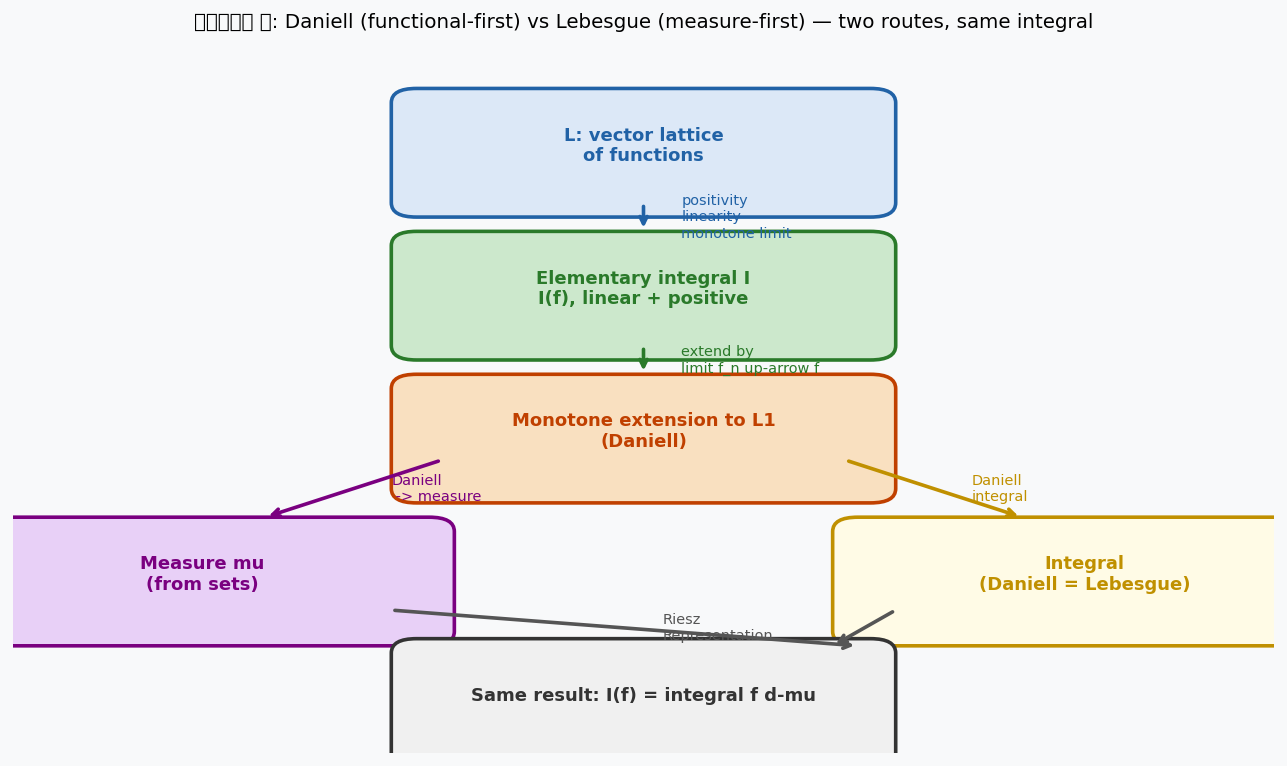
চিত্র ১: Daniell (functional-first, উপর থেকে) ও Lebesgue (measure-first) দুটো পথ। Riesz representation theorem দেখায় এরা একই গন্তব্যে পৌঁছায়।
Vector Lattice — ফাংশনের বীজগণিত
Daniell শুরু করেন একটা বিশেষ ধরনের function space দিয়ে।
Vector lattice (ভেক্টর জালক) \(L\) হলো set \(S\)-এর উপর bounded real-valued functions-এর একটা set যেটা: - vector space: \(f, g \in L \Rightarrow af + bg \in L\) - lattice: \(f, g \in L \Rightarrow f \vee g := \max(f,g) \in L\) এবং \(f \wedge g := \min(f,g) \in L\)
উদাহরণ: \(S = \mathbb{R}^n\), \(L =\) continuous functions of compact support। এটা পুরোপুরি একটা vector lattice।
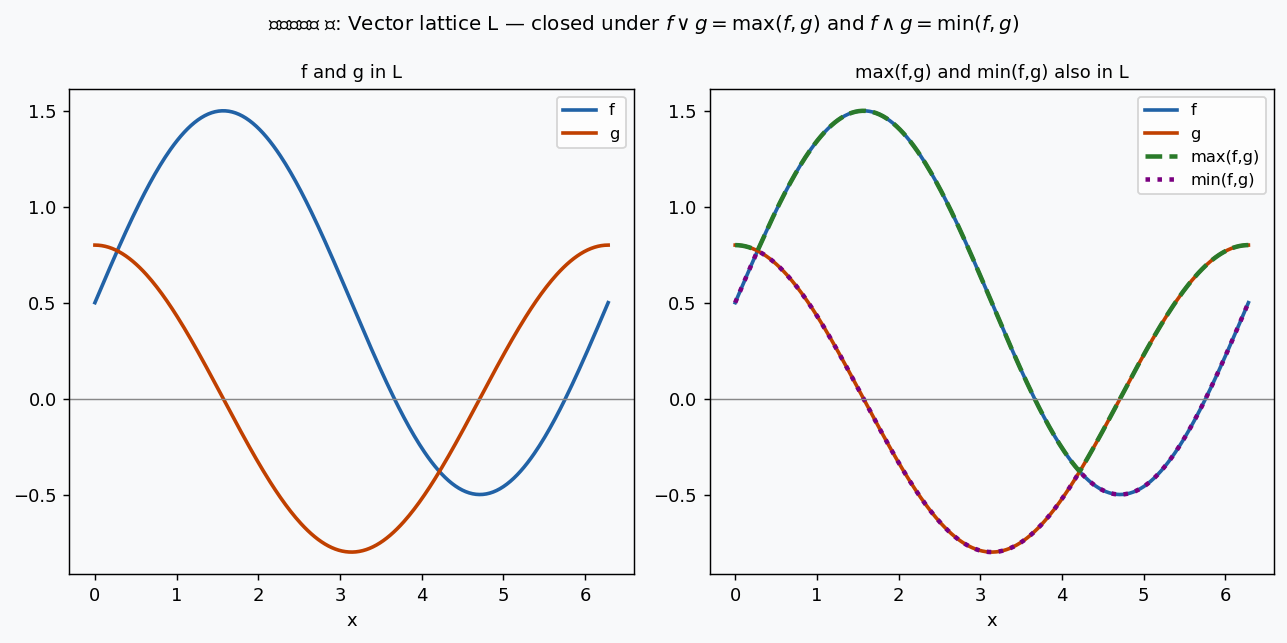
চিত্র ২: বাঁয়ে \(f\) (নীল) ও \(g\) (লাল) দুটো function। ডানে \(\max(f,g)\) (সবুজ, ড্যাশ) ও \(\min(f,g)\) (বেগুনি, বিন্দু) — এরাও \(L\)-এ আছে।
৩. সংজ্ঞা ও উপপাদ্য (Definitions & Theorems)
Elementary Integral — প্রাথমিক ফাংশনাল
সংজ্ঞা (Sternberg 6.1): Daniell Integral
\(L\) একটা vector lattice on \(S\)। একটা map \(I: L \to \mathbb{R}\) কে integral (সমাকল) বলা হয় যদি:
(1) Linearity (রৈখিকতা): \(I(af + bg) = aI(f) + bI(g)\)
(2) Positivity (অ-ঋণাত্মকতা): \(f \geq 0 \Rightarrow I(f) \geq 0\)
(3) Continuity from above: \(f_n \searrow 0 \Rightarrow I(f_n) \searrow 0\)
শর্ত (3)-টাই Daniell integral-এর মূল continuity শর্ত। Dini's lemma থেকে দেখা যায় Riemann integral এই তিনটাই পূরণ করে।
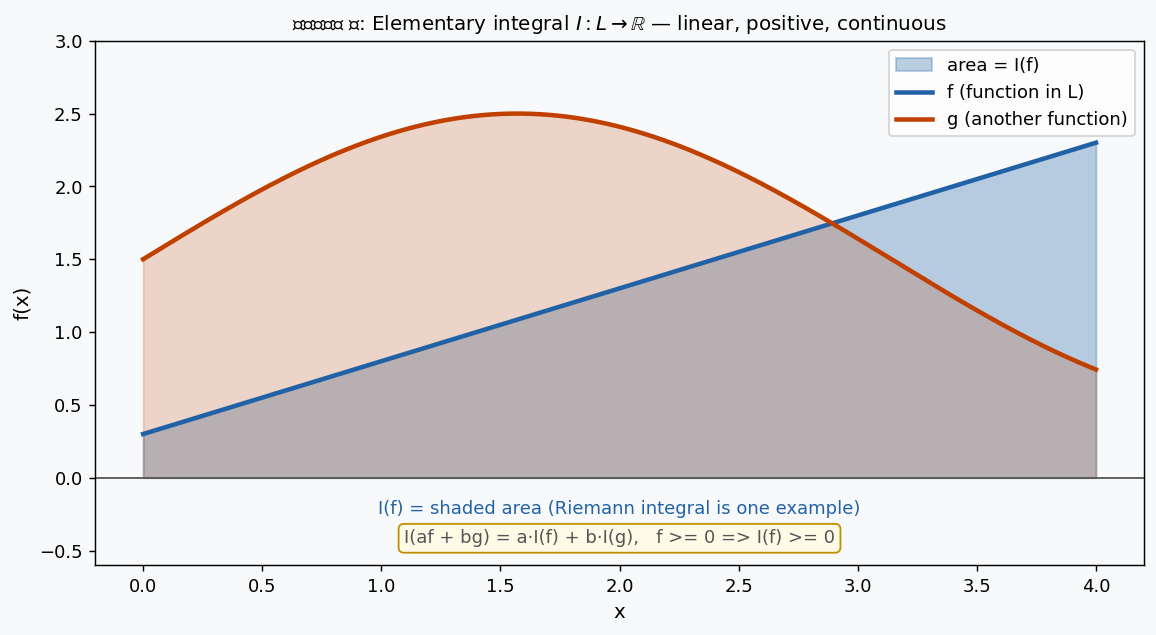
চিত্র ৩: Elementary integral \(I(f)\) হলো \(f\)-এর নিচের shaded area। নীল function \(f\), কমলা function \(g\) — \(I\) তাদের areas দেয়। Positivity: \(f \geq 0 \Rightarrow I(f) \geq 0\)।
Monotone Extension — U এবং L1 তৈরি করা
এখন \(I\) কে ধাপে ধাপে বড় করা হয়।
Step 1: \(U\) তৈরি। \(U := \{\text{limits of monotone non-decreasing sequences from } L\}\)।
অর্থাৎ \(f_n \in L\), \(f_n \nearrow f\) হলে \(f \in U\)।
Lemma (Sternberg 6.1.1–6.1.3): Monotone Extension to U
\(f_n \nearrow f\) হলে \(I(f) := \lim I(f_n)\) সুনির্দিষ্টভাবে define করা যায় — দুটো আলাদা sequence \(f_n \nearrow f\) ও \(g_n \nearrow f\) হলে \(\lim I(f_n) = \lim I(g_n)\)।
আরো: যদি \(h_n \in U\) এবং \(h_n \nearrow h\), তাহলে \(h \in U\) এবং \(I(h_n) \nearrow I(h)\) — এটা \(U\) নিজেই এই limit process-এর অধীনে closed।
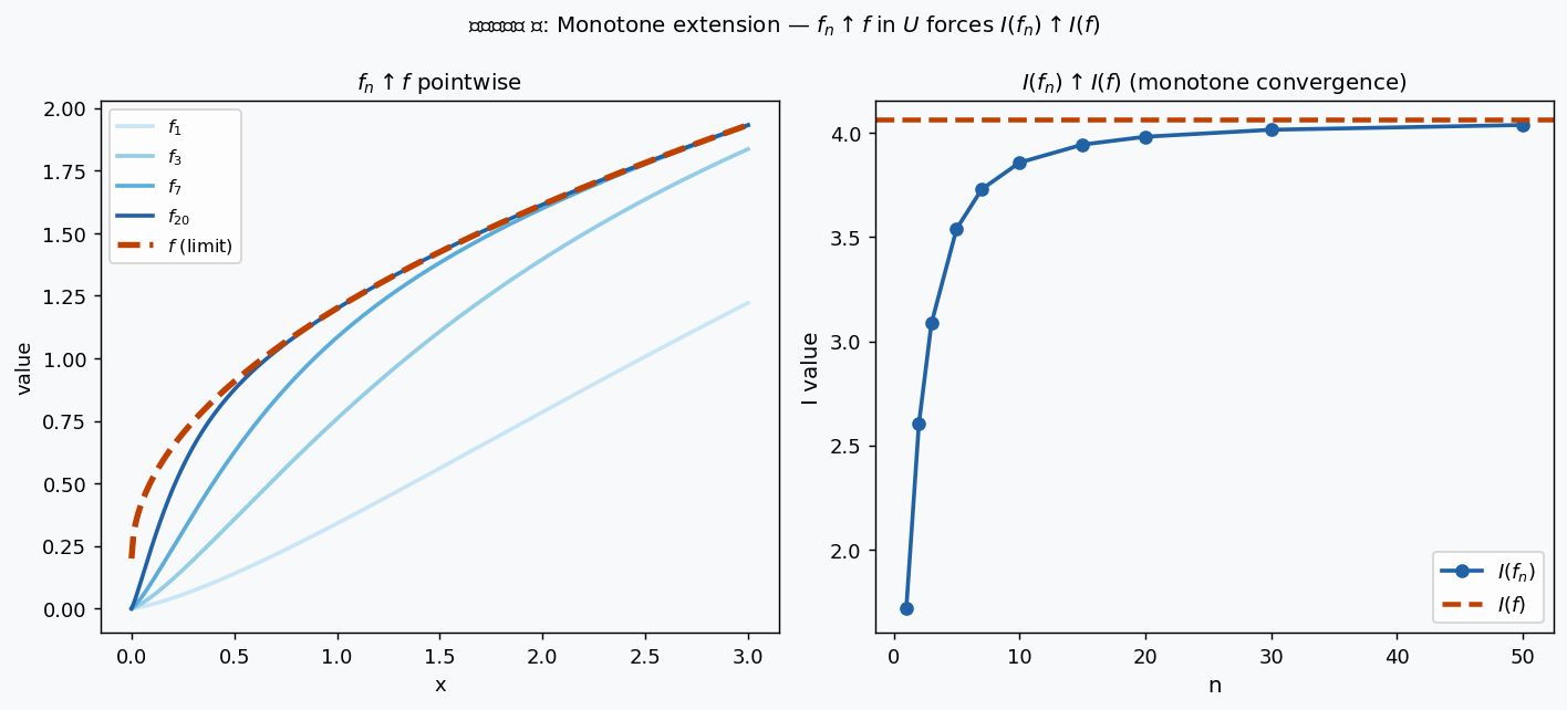
চিত্র ৪: বাঁয়ে \(f_n \nearrow f\) pointwise (রঙ গাঢ় হচ্ছে \(n\) বাড়লে)। ডানে \(I(f_n) \nearrow I(f)\) — integral ও বাড়ছে monotonically। এটাই Daniell-এর MCT (Monotone Convergence Theorem)।
Step 2: Summable functions। \(f\) কে \(I\)-summable বলা হয় যদি প্রতিটা \(\varepsilon > 0\) এর জন্য \(g \in -U\), \(h \in U\) পাওয়া যায় যেন \(g \leq f \leq h\) এবং \(I(h - g) \leq \varepsilon\)।
এই summable functions-এর space কে বলা হয় \(L^1\)।
Theorem 6.1.1 (Sternberg): Daniell Monotone Convergence Theorem
\(f_n \in L^1\), \(f_n \nearrow f\), এবং \(\lim I(f_n) < \infty\) হলে \(f \in L^1\) এবং:
এটা Lebesgue-এর Monotone Convergence Theorem-এর অবিকল সমতুল্য — শুধু এখানে আমরা measure ছাড়াই পেলাম।
Daniell Integral থেকে Measure
এখন একটা আশ্চর্য ঘটনা: Daniell integral থেকে সরাসরি measure বের করা যায়।
Section 6.3 (Sternberg): Measure from Daniell Integral
যোগ করো Stone's axiom: \(f \in L \Rightarrow f \wedge 1 \in L\)।
তাহলে: একটা set \(A\) কে integrable বলা হয় যদি \(\mathbf{1}_A \in B\) (Borel class)। এই integrable sets একটা \(\sigma\)-field গঠন করে।
সংজ্ঞা করো:
Daniell-এর MCT গ্যারান্টি দেয় যে \(\mu\) একটা countably additive measure।
আরো: \(f \in L^1\) হলে \(I(f) = \int f\, d\mu\)।
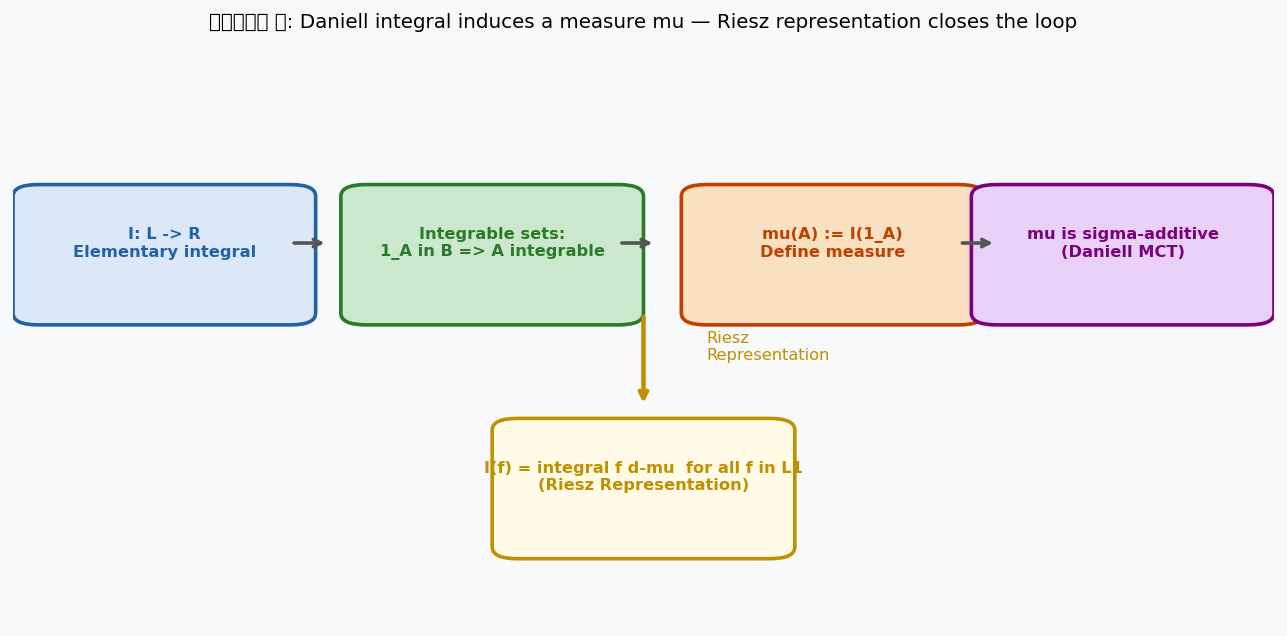
চিত্র ৫: Daniell integral \(I\) থেকে measure \(\mu\) বের করার ধাপগুলো। Riesz representation theorem চূড়ান্তভাবে বলে \(I(f) = \int f\, d\mu\) সব \(f \in L^1\)-এর জন্য।
Positivity Axiom — কেন জরুরি
Positivity এবং তার পরিণতি
\(f \geq 0 \Rightarrow I(f) \geq 0\)।
এর ফলে: \(f \leq g \Rightarrow I(f) \leq I(g)\) (monotonicity)।
আরো: \(I(f^+) \geq 0\) এবং \(I(f^-) \geq 0\) যেখানে \(f^+ = \max(f,0)\) ও \(f^- = \max(-f,0)\)।
যেকোনো \(f\) কে positive ও negative part-এ ভাগ করা যায়: \(f = f^+ - f^-\)।
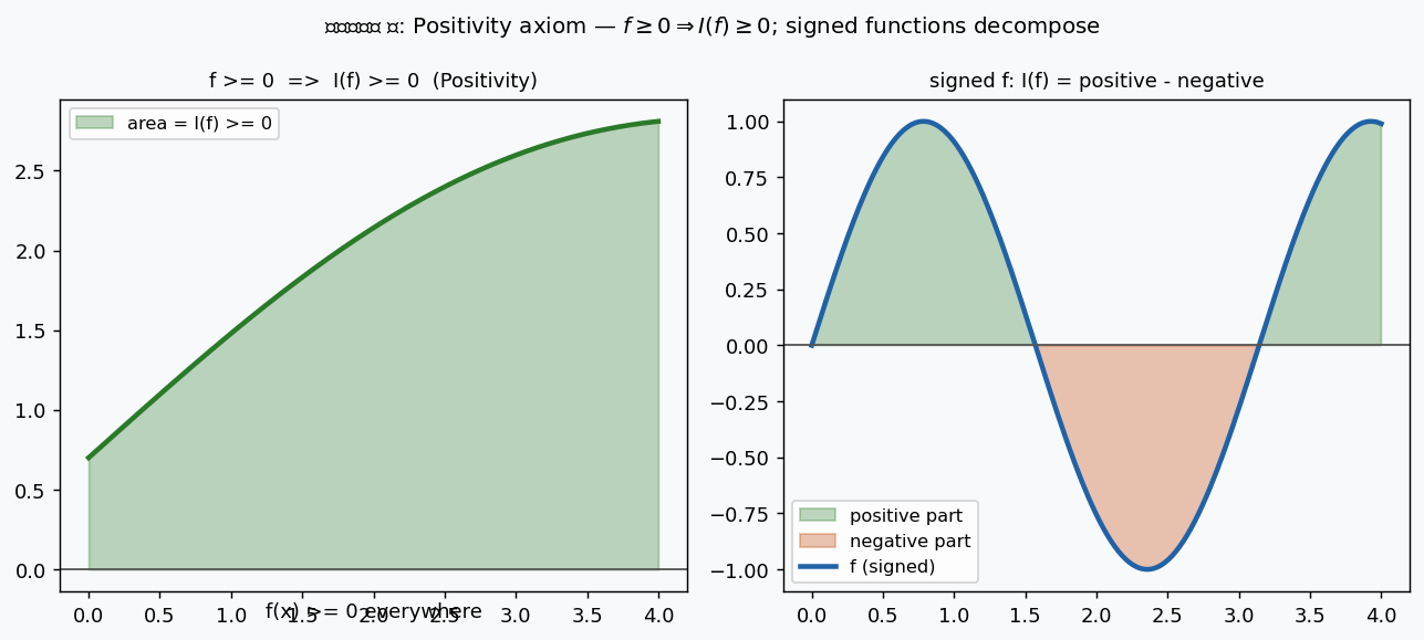
চিত্র ৬: বাঁয়ে \(f \geq 0\) সর্বত্র — \(I(f) \geq 0\)। ডানে signed function: সবুজ ছায়া = positive part \(I(f^+)\), লাল ছায়া = negative part \(I(f^-)\); \(I(f) = I(f^+) - I(f^-)\)।
Daniell ↔ Lebesgue: সমতুল্যতা
এই দুটো পদ্ধতি একে অপরের সমতুল্য — proof টা Riesz representation theorem-এর মাধ্যমে আসে।
Theorem 6.8.1 (Sternberg): Riesz Representation via Daniell
\(X\) locally compact Hausdorff space হোক, \(L = C_c(X)\) (compact support-এর continuous functions)।
যেকোনো non-negative linear functional \(I: L \to \mathbb{R}\) স্বয়ংক্রিয়ভাবে একটা Daniell integral (তিনটা axiom পূরণ করে, Dini's lemma থেকে)।
Riesz Representation Theorem (উন্নত রূপ): এমন একটা \(\sigma\)-field \(\mathcal{F} \supseteq \mathcal{B}(X)\) এবং regular measure \(\mu\) আছে যেন:
এবং \(\mu\!\restriction_{\mathcal{B}(X)}\) unique।
এই theorem-টার মানে: locally compact Hausdorff space-এ "ভালো" linear functional = measure। দুটো পথ একটাই।
Radon-Nikodym Daniell-style (Section 6.6): যদি \(I\) ও \(J\) দুটো bounded integral এবং \(J\) absolutely continuous w.r.t. \(I\) হয়, তাহলে:
প্রমাণটা চমৎকার: \(K = I + J\) নিয়ে \(L^2(K)\) Hilbert space-এ Riesz representation theorem প্রয়োগ করলে \(f_0\) পাওয়া যায় — functional analysis-ই এখানে measure theory produce করছে।
৪. উদাহরণ ও Analogy
উদাহরণ ১: Riemann Integral থেকে Lebesgue পর্যন্ত
\(S = [0,1]\), \(L = C([0,1])\) (continuous functions)।
\(I(f) = \int_0^1 f(x)\, dx\) (Riemann integral)।
তিনটা axiom সহজেই verify হয় — Dini's lemma দেয় axiom (3)।
Daniell-এর procedure চালালে পাওয়া যায় \(\mu = \lambda\) (Lebesgue measure) এবং \(I\) extend হয় Lebesgue integral-এ। অর্থাৎ Riemann integral থেকে Daniell procedure চালালে Lebesgue integral পাওয়া যায়।
উদাহরণ ২: \(L^p\) Theory — ভিতর থেকে
Sternberg Section 6.4-এ Hölder's ও Minkowski's inequality Daniell framework-এ prove করা হয়েছে:
আর \(L^p\) complete হওয়ার (Banach space) প্রমাণও Daniell framework-এ সহজ — এটা দেখায় যে Daniell পদ্ধতি \(L^p\) theory-কে আরো স্বাভাবিকভাবে build করে।
উদাহরণ ৩: Haar Measure
Locally compact groups (যেমন \(\mathbb{R}^n\), \(SO(3)\), \(GL_n(\mathbb{R})\)) এর উপর translation-invariant integral define করতে Daniell পদ্ধতি ব্যবহার হয় — প্রথমে \(L = C_c(G)\)-এ invariant functional, তারপর Riesz দিয়ে Haar measure।
Analogy: দুটো রাস্তায় একই পাহাড়চূড়া
কল্পনা করো দুটো পর্বতারোহী দল। একটা দল ট্রেইল ম্যাপ দিয়ে শুরু করে (measure first); অন্য দল শুধু কম্পাস ও altitude sensor নিয়ে শুরু করে (integral first)। দুটো দলই একই শিখরে পৌঁছায়। শিখরটা হলো "সম্পূর্ণ integration theory"।
Daniell পদ্ধতিটা বিশেষ কাজের যখন "ম্যাপ" (measure) সরাসরি পাওয়া কঠিন — কিন্তু "altitude" (integral) সহজে মাপা যায়।
৫. সাধারণ ভুল (Common mistakes)
-
Axiom (3) ছাড়া Daniell integral হয় না। Linearity ও positivity থাকলেও axiom (3) (\(f_n \searrow 0 \Rightarrow I(f_n) \searrow 0\)) ছাড়া extension কাজ করে না। এটাই Riemann integral-কে Daniell integral বানায়।
-
Stone's axiom ছাড়া measure নাও পাওয়া যেতে পারে। \(f \in L \Rightarrow f \wedge 1 \in L\) না হলে \(\mathbf{1}_A\)-type functions গড়া যায় না।
-
\(I\) ও \(\int d\mu\) সবসময় equal নয় শুরুতে। Daniell procedure-এ \(I\) প্রথমে শুধু \(L\)-এ define। Extension-এর পর \(I(f) = \int f\, d\mu\) হয় \(L^1\)-এর সব \(f\) এর জন্য — শুধু \(L\)-এর নয়।
-
Daniell "সহজ" ভাবা। মূল construction — U, \(-U\), summability — বেশ সূক্ষ্ম। Monotone class theorem-এর কাজ আছে।
-
\(B\) class ও \(L^1\) class গুলিয়ে ফেলা। Sternberg-এ \(B\) হলো smallest monotone class containing \(L\); \(L^1 = L^1 \cap B\) হলো integrable functions। \(B\) বড়, \(L^1\) ছোট (finite integral-এর শর্ত আছে)।
-
Riesz measure সবসময় Lebesgue measure নয়। Riesz representation দেয় একটা regular Borel measure; কিন্তু কোন measure সেটা নির্ভর করে \(I\)-এর উপর। \(I =\) Riemann integral দিলে Lebesgue measure; অন্য \(I\) হলে অন্য measure।
৬. এক্সারসাইজ (Exercises)
নিজে চেষ্টা করো, তারপর সমাধান খোলো।
-
\(L = C([0,1])\), \(I(f) = f(0) + f(1)\) (boundary functional)। তিনটা axiom verify করো। এই \(I\) কোন measure \(\mu\)-র সাথে correspond করে?
-
\(L = C([0,1])\), \(I(f) = \int_0^1 f(x) x\, dx\) (weighted Riemann)। Daniell পদ্ধতি চালালে কোন measure \(\mu\) পাওয়া যাবে? \(\mu([0, t]) = ?\)
-
দেখাও যে \(f_n = \mathbf{1}_{[1/n, 1]}\) on \([0,1]\) হলে \(f_n \nearrow \mathbf{1}_{(0,1]}\)। Riemann integral \(I(f_n) = 1 - 1/n \nearrow 1\)। এই example দিয়ে Daniell extension কীভাবে কাজ করে বোঝাও।
-
\(S = \mathbb{Z}\), \(L = c_{00}\) (finite support sequences), \(I(f) = \sum_{n \in \mathbb{Z}} f(n)\)। তিনটা axiom verify করো। এই \(I\) কোন measure correspond করে?
-
Daniell framework-এ দেখাও: \(I(f \vee g) + I(f \wedge g) = I(f) + I(g)\) সব \(f, g \in L\)-এর জন্য।
-
Radon-Nikodym Daniell-style: ধরো \(I(f) = \int_0^1 f\, d\lambda\) এবং \(J(f) = \int_0^1 f(x) \cdot 2x\, d\lambda(x)\)। \(f_0\) খোঁজো যেন \(J(f) = I(f \cdot f_0)\)।
-
Stone's axiom ছাড়া Daniell-কে counter-example দিয়ে ব্যর্থ করো: \(L =\) linear functions on \(\mathbb{R}\) (polynomials of degree \(\leq 1\)), \(I(ax+b) = b\)। Stone's axiom ব্যর্থ হয় কীভাবে? Indicator function গড়া যায় না কেন?
৭. সমাধান (ব্যাখ্যাসহ)
১-নং সমাধান দেখাও
\(I(f) = f(0) + f(1)\)।
Linearity: \(I(af+bg) = (af+bg)(0) + (af+bg)(1) = a(f(0)+f(1)) + b(g(0)+g(1)) = aI(f)+bI(g)\) ✓
Positivity: \(f \geq 0 \Rightarrow f(0) \geq 0\) এবং \(f(1) \geq 0\), তাই \(I(f) \geq 0\) ✓
Axiom (3): \(f_n \searrow 0\) pointwise, continuous functions on compact set, তাই uniform → \(f_n(0), f_n(1) \searrow 0\), তাই \(I(f_n) \searrow 0\) ✓
Corresponding measure: \(\mu = \delta_0 + \delta_1\) (point masses at \(0\) and \(1\))।
২-নং সমাধান দেখাও
\(I(f) = \int_0^1 f(x) x\, d\lambda(x)\)।
Linearity ও positivity সহজ। Axiom (3): \(f_n \searrow 0\) uniformly on \([0,1]\) (Dini) → \(I(f_n) = \int f_n(x) x\, dx \searrow 0\) ✓
Corresponding measure: \(d\mu = x\, d\lambda\), অর্থাৎ \(\mu(A) = \int_A x\, d\lambda(x)\)।
Distribution function: \(\mu([0,t]) = \int_0^t x\, dx = \frac{t^2}{2}\) এবং density \(h(x) = x\) on \([0,1]\)।
এটা uniform নয় — \([0,t]\)-এর weight \(\frac{t^2}{2}\), সুতরাং কাছের points কম weighted।
৩-নং সমাধান দেখাও
\(f_n = \mathbf{1}_{[1/n,1]} \in L\) (continuous? না — piecewise constant; তাই ধরো \(f_n\) continuous approximation যা \([1/n,1]\)-এ \(1\), কিছুটা smooth করা)।
\(f_n \nearrow \mathbf{1}_{(0,1]}\) pointwise সব \(x \in (0,1]\)-এর জন্য।
Riemann: \(I(f_n) = \int_0^1 f_n\, dx \approx 1 - 1/n \nearrow 1\)।
Daniell extension: \(\mathbf{1}_{(0,1]} \in U\) (limit of increasing sequence from \(L\))।
\(I(\mathbf{1}_{(0,1]}) = \lim I(f_n) = 1 = \lambda((0,1])\) ✓।
এই example দেখায় Daniell extension Riemann integral-কে স্বয়ংক্রিয়ভাবে extend করে non-continuous functions-এ।
৪-নং সমাধান দেখাও
\(I(f) = \sum_{n \in \mathbb{Z}} f(n)\) on \(c_{00}\) (finite support sequences)।
Linearity: সরাসরি series-এর linearity থেকে ✓
Positivity: \(f \geq 0 \Rightarrow\) সব terms \(\geq 0 \Rightarrow\) sum \(\geq 0\) ✓
Axiom (3): \(f_k \searrow 0\) on \(\mathbb{Z}\), finite support (all supported in \(\{-N,...,N\}\) for some \(N\)) → \(f_k(n) \searrow 0\) each \(n\) → \(I(f_k) = \sum_n f_k(n) \searrow 0\) ✓
Corresponding measure: \(\mu =\) counting measure on \(\mathbb{Z}\) — \(\mu(A) = \lvert A\rvert\)।
\(I(f) = \sum_{n} f(n) = \int f\, d\mu_\text{counting}\) ✓।
৫-নং সমাধান দেখাও
\(f \vee g = \max(f,g) = \frac{f+g+\lvert f-g\rvert}{2}\) এবং \(f \wedge g = \frac{f+g-\lvert f-g\rvert}{2}\)।
তাই:
\(I\) linear হওয়ায়:
এটা probability theory-তে inclusion-exclusion formula-র analog।
৬-নং সমাধান দেখাও
\(I(f) = \int_0^1 f\, d\lambda\), \(J(f) = \int_0^1 2xf(x)\, d\lambda(x)\)।
Radon-Nikodym: \(J(f) = I(f \cdot f_0)\) মানে:
তুলনা করে: \(f_0(x) = 2x\)।
Verify: \(I(f \cdot f_0) = \int_0^1 f(x) \cdot 2x\, dx = J(f)\) ✓।
এটা Radon-Nikodym থেকে আসে: \(J\) absolutely continuous w.r.t. \(I\) (কারণ \(J(f) \leq 2\lVert f\rVert_\infty \cdot I(\mathbf{1}) = 2I(f)\) for \(f \geq 0\)), তাই \(f_0 = d\mu_J/d\mu_I = 2x\)।
৭-নং সমাধান দেখাও
\(L = \{ax + b : a, b \in \mathbb{R}\}\), \(I(ax+b) = b\)।
Stone's axiom: \(f \in L \Rightarrow f \wedge 1 \in L\)?
\(f(x) = 2x\) নিই। তাহলে \((2x) \wedge 1 = \min(2x, 1)\)।
এটা \(x \leq 1/2\)-এ \(2x\), \(x > 1/2\)-এ \(1\) — পiecewise linear কিন্তু linear নয় (\(L\)-এর বাইরে)। Stone's axiom fails ✓
Indicator function গড়া যায় না: \(\mathbf{1}_{[0,1/2]}\) গড়তে হলে \(f_n \nearrow \mathbf{1}_{[0,1/2]}\) এমন sequence চাই \(L\)-এ — কিন্তু linear functions কোনো bounded set-এর indicator-এ converge করতে পারে না। তাই \(\mu([0,1/2])\) define হয় না, Daniell-থেকে-measure construction ব্যর্থ।
এটাই দেখায় Stone's axiom ছাড়া Daniell integral measure theory produce করতে পারে না।
৮. সারসংক্ষেপ ও Checklist
এই অধ্যায়ের পর নিজেকে যাচাই করো:
- [ ] Daniell integral-এর তিনটা axiom জানি: linearity, positivity, \(f_n \searrow 0 \Rightarrow I(f_n) \searrow 0\)।
- [ ] Vector lattice \(L\) বুঝি — \(\max\) ও \(\min\)-এর অধীনে closed।
- [ ] Monotone extension জানি: \(f_n \nearrow f\) হলে \(I(f) := \lim I(f_n)\) সুনির্দিষ্ট।
- [ ] Daniell MCT: \(f_n \nearrow f\), bounded \(\Rightarrow I(f) = \lim I(f_n)\)।
- [ ] Stone's axiom কী এবং কেন দরকার — indicator function গড়তে।
- [ ] \(\mu(A) = I(\mathbf{1}_A)\) দিয়ে কীভাবে measure পাওয়া যায় জানি।
- [ ] Daniell ↔ Lebesgue সমতুল্যতা বুঝি: Riesz representation theorem-এর মাধ্যমে।
- [ ] Radon-Nikodym Daniell-style: \(J = I(f_0 \cdot)\) form।
➡️ পরের অধ্যায়: 7.3 — Wiener Measure ও Brownian Motion — Daniell-এর framework ব্যবহার করে অসীম-মাত্রিক path space \(C([0,1])\) এর উপর একটা measure define করা যায় — এটাই Wiener measure, এবং এর সাথে আসে Brownian motion।