7.3 — Wiener Measure ও Brownian Motion¶

এই অধ্যায়ে কী শিখব: Brownian motion (এলোমেলো অবিচ্ছিন্ন গতি) কী এবং কোথা থেকে আসে; Wiener measure — continuous path-দের space \(C[0,\infty)\)-এর উপর একটি probability measure; পথের মূল বৈশিষ্ট্য — সর্বত্র continuous কিন্তু কোথাও differentiable নয়; Gaussian independent increments; scaling invariance (\(\sqrt{t}\) spreading); white noise — Brownian motion-এর distributional derivative।

উৎস (source): Robert Brown, Einstein, Wiener।

১. কেন শিখব? (Motivation)¶

১৮২৭ সালে botanist (উদ্ভিদবিজ্ঞানী) Robert Brown একটি মাইক্রোস্কোপে পানিতে ভাসমান পরাগকণা দেখছিলেন। কণাগুলো একদম এলোমেলোভাবে নাচছিল — কোনো দিকনির্দেশনা নেই, থামছে না, কোনো নিয়ম মেনে চলছে না। এই ঘটনাটাকে বলা হলো Brownian motion (ব্রাউনীয় গতি)।

Albert Einstein ১৯০৫ সালে এটা ব্যাখ্যা করলেন: কণাটাকে অণু-পরমাণু অগণিতবার ধাক্কা মারছে — প্রতিটা ধাক্কা স্বাধীন, ক্ষুদ্র, যেকোনো দিকে। Central limit theorem বলে এত অনেক স্বাধীন ধাক্কার সম্মিলিত ফল হবে Gaussian।

কিন্তু এটাকে rigorous mathematics-এ ধরা কঠিন ছিল। Norbert Wiener ১৯২৩ সালে সেই কাজটা করলেন — continuous path-দের বিশাল space-এর উপর একটা probability measure তৈরি করলেন, যাকে বলা হয় Wiener measure (উইনার পরিমাপ)।

কেন এটা গুরুত্বপূর্ণ?

Finance (অর্থনীতি): শেয়ারের দাম Brownian motion মেনে চলে বলে ধরা হয় — Black-Scholes formula সেই ভিত্তিতে।
Physics: heat diffusion (তাপ ছড়িয়ে পড়া), quantum path integrals — সব Brownian motion-এর ভাষায়।
Statistics: white noise (সাদা শব্দ) হলো signal processing-এর মূল ধারণা।
Mathematics: Wiener measure হলো infinite-dimensional space-এর উপর measure তৈরির প্রথম বড় উদাহরণ।

মূল স্বজ্ঞা

Random walk-এ প্রতি সেকেন্ডে এক পদক্ষেপ। পদক্ষেপের size ছোট করো, সংখ্যা বাড়াও — limit-এ Brownian motion পাওয়া যায়। Wiener measure হলো এই limit-এর rigorous version।

২. মূল ধারণা (Core idea)¶

Random Walk থেকে Brownian Motion¶

ভাবো একটা particle এক মাত্রায় হাঁটছে। প্রতি \(\frac{1}{n}\) সময়ে সে \(+\frac{1}{\sqrt{n}}\) বা \(-\frac{1}{\sqrt{n}}\) যাচ্ছে — সমান সম্ভাবনায়, স্বাধীনভাবে। \(n\) বড় হলে কী হয়?

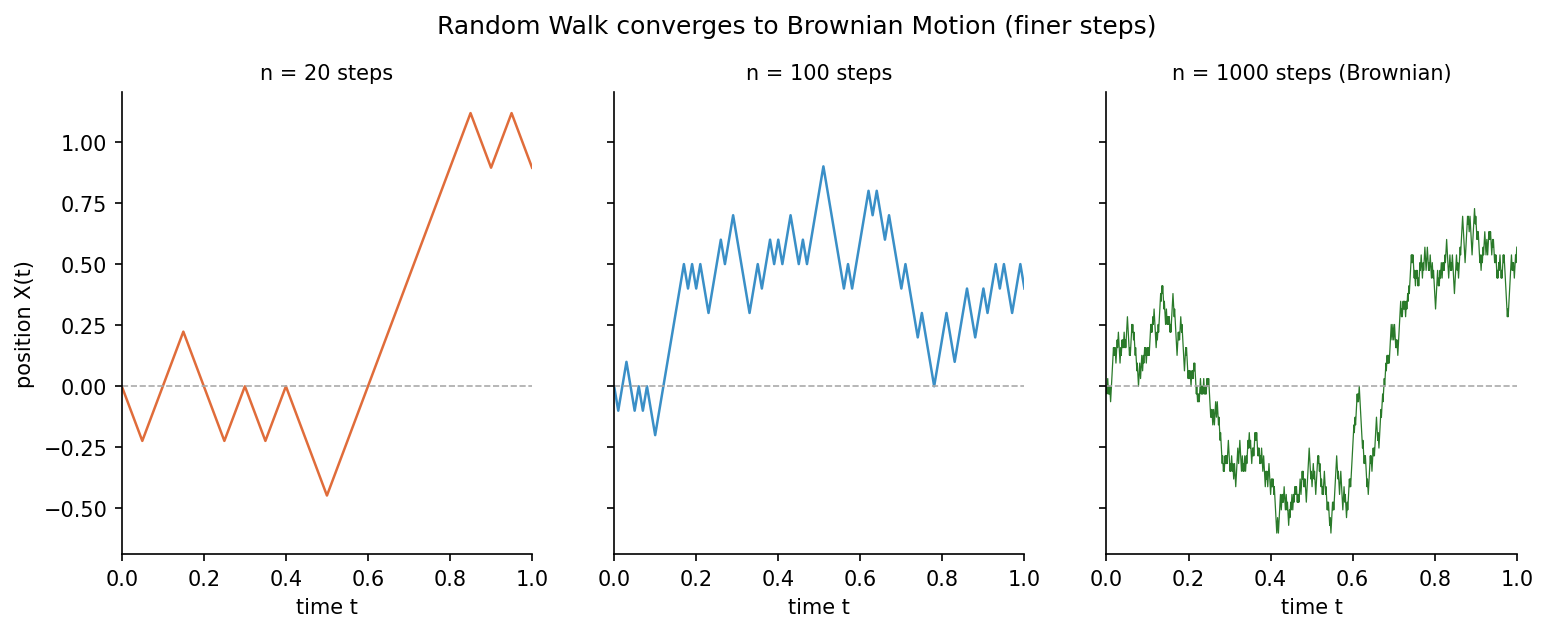
Random walk converges to Brownian motion

চিত্র ১: \(n=20\), \(100\), \(1000\) পদক্ষেপের random walk। পদক্ষেপ সূক্ষ্ম হলে path smooth নয়, বরং তীব্রভাবে jagged — এটাই Brownian motion-এর characteristic।

\(n \to \infty\) হলে এই random walk-গুলো একটি limiting process-এ converge করে — সেটাই Brownian motion \(\{B_t\}_{t \geq 0}\)।

Brownian Motion-এর বৈশিষ্ট্য¶

Brownian motion-এর চারটা মূল বৈশিষ্ট্য:

\(B_0 = 0\) (origin থেকে শুরু)
Continuous paths: প্রতিটি sample path \(t \mapsto B_t(\omega)\) একটি continuous function
Independent increments (স্বাধীন বৃদ্ধি): \(s < t < u < v\) হলে \(B_t - B_s\) এবং \(B_v - B_u\) স্বাধীন
Gaussian increments: \(B_t - B_s \sim N(0,\, t-s)\) — অর্থাৎ \(t-s\) দৈর্ঘ্যের ব্যবধানে displacement হলো mean 0, variance \(t-s\)-এর Gaussian

Six independent Brownian paths

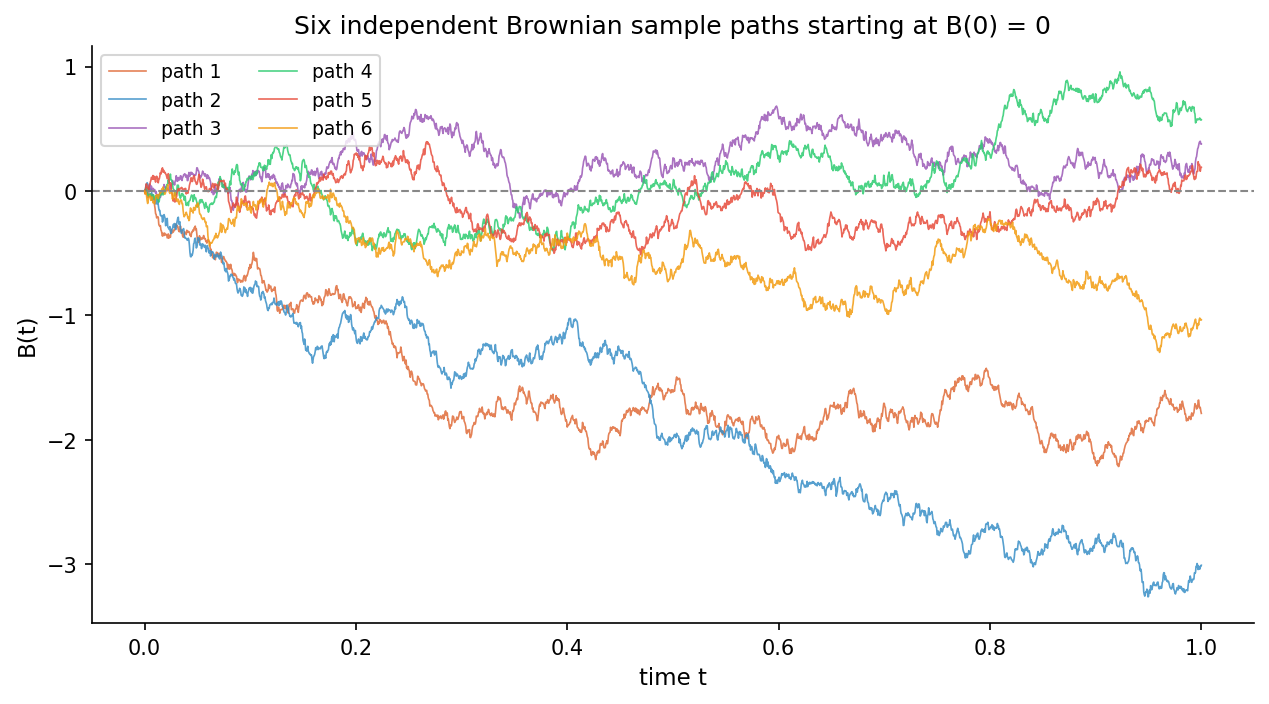
চিত্র ২: ছয়টি স্বাধীন Brownian sample path। সবগুলো \(B_0 = 0\) থেকে শুরু। প্রতিটি ভিন্ন — path space-এ uncountably many path আছে।

৩. সংজ্ঞা ও উপপাদ্য (Definitions & Theorems)¶

Brownian Motion-এর সংজ্ঞা¶

সংজ্ঞা ৭.১ (Brownian Motion)

একটি stochastic process (এলোমেলো প্রক্রিয়া) \(\{B_t\}_{t \geq 0}\) কে standard Brownian motion বলা হয় যদি:

(a) \(B_0 = 0\) প্রায় নিশ্চিতভাবে (almost surely)

(b) যেকোনো \(0 \leq s < t\)-এর জন্য, increment (বৃদ্ধি):

\[B_t - B_s \;\sim\; N(0,\; t-s)\]

(c) Increments স্বাধীন: \(0 \leq t_0 < t_1 < \cdots < t_k\)-এর জন্য \(B_{t_1} - B_{t_0},\; B_{t_2} - B_{t_1},\; \ldots,\; B_{t_k} - B_{t_{k-1}}\) পরস্পর স্বাধীন

(d) প্রায় সব \(\omega\)-এর জন্য \(t \mapsto B_t(\omega)\) একটি continuous function

Gaussian increment মানে: যদি \(t - s = 0.5\) হয়, তাহলে displacement-এর density হলো \(\frac{1}{\sqrt{\pi}}\,e^{-x^2}\)। ব্যবধান ছোট হলে bell curve সরু, বড় হলে চওড়া।

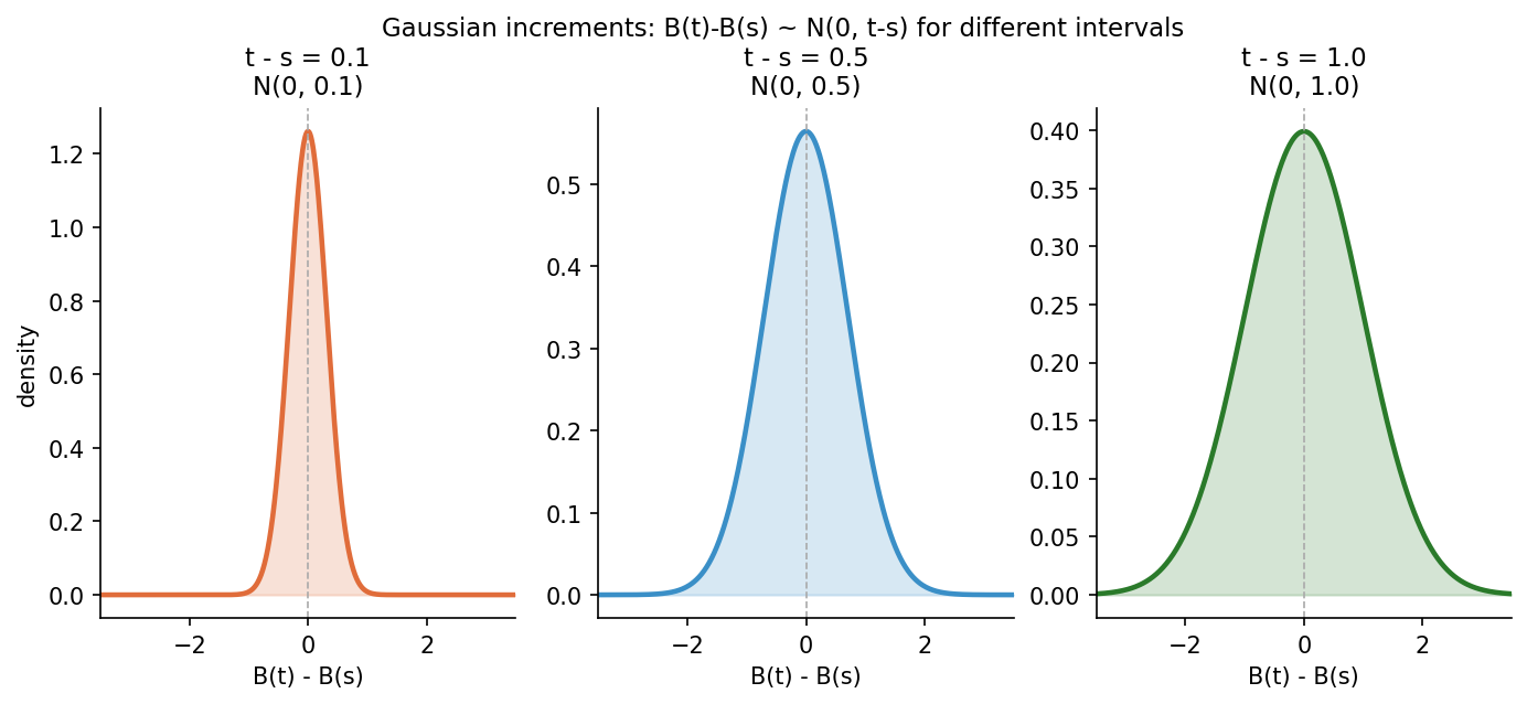
Gaussian increments for different interval lengths

চিত্র ৩: \(t-s = 0.1\), \(0.5\), \(1.0\)-এর জন্য \(B_t - B_s\)-এর distribution। ব্যবধান বড় হলে spread বাড়ে — variance \(= t-s\)।

Wiener Measure¶

Wiener measure (উইনার পরিমাপ) \(W\) বা \(\text{pr}_0\) হলো continuous path-দের space-এর উপর একটি probability measure। সেই space টা হলো:

\[C[0,\infty) := \{\omega : [0,\infty) \to \mathbb{R} \mid \omega \text{ continuous}, \omega(0) = 0\}\]

Wiener measure নির্মাণ হয় Nelson-এর পদ্ধতিতে: প্রথমে finite-dimensional distributions নির্ধারণ করো (finite set of times \(t_1 < t_2 < \cdots < t_m\)-এ path কোথায় যাবে তার joint probability), তারপর Riesz representation theorem দিয়ে সেটাকে \(C[0,\infty)\)-এর উপর একটা regular Borel measure-এ extend করো।

Sternberg-এর গঠন অনুযায়ী, path \(\omega\) যদি \(E_i\)-তে সময় \(t_i\)-তে থাকার probability:

\[W(E) = \int_{E_1} \cdots \int_{E_m} p(0,x_1;\,t_1)\, p(x_1,x_2;\,t_2-t_1)\, \cdots\, p(x_{m-1},x_m;\,t_m-t_{m-1})\; dx_1 \cdots dx_m\]

যেখানে heat kernel (তাপ কার্নেল) হলো:

\[p(x,y;\,t) = \frac{1}{\sqrt{2\pi t}}\, e^{-(x-y)^2/(2t)}\]

উপপাদ্য ৭.১ (Wiener, ১৯২৩)

Wiener measure \(W\) প্রায় নিশ্চিতভাবে continuous path-দের উপর concentrate (কেন্দ্রীভূত) থাকে:

\[W(C[0,\infty)) = 1\]

অর্থাৎ discontinuous path-দের Wiener measure শূন্য।

প্রমাণ-স্কেচ: Kolmogorov continuity criterion ব্যবহার করে দেখানো যায়: যেকোনো \(\epsilon > 0\) এবং interval \([a,b]\)-এর জন্য, \(\lvert B_s - B_t\rvert > 4\epsilon\) হওয়ার probability \(\leq 2\rho(\frac{1}{2}\epsilon, \delta)\) যেখানে \(\rho(\epsilon, \delta) \to 0\) as \(\delta \to 0\)। তাই discontinuous path-দের set-এর measure শূন্য। \(\square\)

Nowhere Differentiable¶

Brownian path-দের সবচেয়ে মজার বৈশিষ্ট্য: continuous হওয়া সত্ত্বেও কোথাও differentiable নয়।

উপপাদ্য ৭.২ (Nowhere Differentiability)

Wiener measure 1-এ, Brownian motion \(B_t\) প্রায় কোনো \(t\)-তেই differentiable নয়।

স্বজ্ঞা: যেকোনো বিন্দুতে \(h \to 0\) হলে \(\frac{B_{t+h} - B_t}{h}\) converge করে না — বরং এর variance \(= \frac{1}{h} \to \infty\)। এটা zoom করলেও ঠিক একই রকম jagged থাকে (self-similar)।

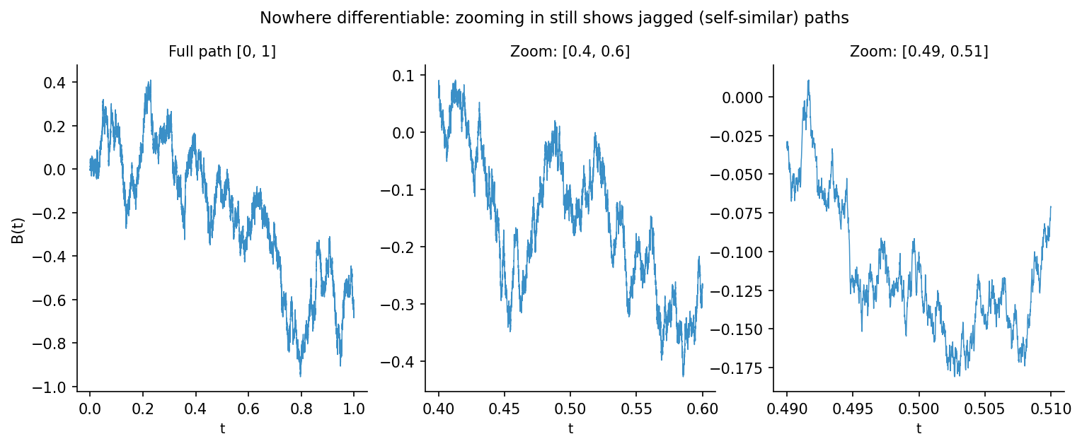
Nowhere differentiable: zoom reveals same jaggedness

চিত্র ৪: Full path \([0,1]\), তারপর \([0.4, 0.6]\), তারপর \([0.49, 0.51]\)-এ zoom। প্রতিটা zoom-এ একই রকম jagged — কোনো smooth tangent নেই।

৪. Scaling Invariance ও Path Space¶

\(\sqrt{t}\) Scaling¶

\[\text{Var}(B_t) = t \implies \text{std}(B_t) = \sqrt{t}\]

এর মানে: সময় \(t\)-তে particle-টা origin থেকে কতদূর যেতে পারে তার typical scale হলো \(\sqrt{t}\) — linear নয়, বরং sublinear।

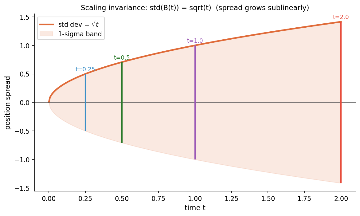
Square-root scaling of Brownian spread

চিত্র ৫: \(\sqrt{t}\) scaling — সময়ের সাথে Brownian motion-এর spread বাড়ে, কিন্তু \(t\)-এর বদলে \(\sqrt{t}\)-এর হারে। orange = \(\pm\sqrt{t}\) band।

Scaling invariance আরো গভীর: যদি \(c > 0\) হয়, তাহলে

\[\{c^{-1/2} B_{ct}\}_{t \geq 0} \overset{d}{=} \{B_t\}_{t \geq 0}\]

অর্থাৎ time rescale করলে যে Brownian motion পাওয়া যায়, সেটা original-এর মতোই distributed।

Wiener Measure on Path Space¶

Wiener measure-কে visualize করতে ভাবো যে আমরা \(C[0,1]\) — সব continuous path-দের একটা বিশাল space — নিয়ে কাজ করছি। Wiener measure এই space-এ events-কে probability দেয়।

Wiener measure on path space C[0,1]

চিত্র ৬: Wiener measure on \(C[0,1]\)। প্রতিটি রঙিন curve একটি sample path। Blue dashed band = \(\pm\sqrt{t}\) (1-sigma)। Box annotation: \(W(E)\) = event \(E\) (নির্দিষ্ট region-এ যাওয়ার) probability।

Heat Equation সংযোগ

Heat kernel \(p(x,y;t)\) হলো heat equation (তাপ সমীকরণ)-এর fundamental solution:

\[\frac{\partial u}{\partial t} = \frac{1}{2}\frac{\partial^2 u}{\partial x^2}, \quad u(0,x) = f(x)\]

solution হলো \(u(t,x) = \int p(x,y;t)\,f(y)\,dy\)। তাই Brownian motion এবং heat diffusion একই গণিত ভাষায় কথা বলে।

৫. Gaussian Measures ও White Noise¶

Centered Gaussian Process¶

\(B_t\)-এর উপর test function \(\phi\) integrate করলে পাওয়া যায়:

\[\langle B, \phi \rangle = \int_0^\infty B_t\, \phi(t)\, dt\]

এটা একটা centered Gaussian random variable যার variance:

\[\text{Var}(\langle B, \phi \rangle) = \int_0^\infty \int_0^\infty \min(s,t)\, \phi(s)\, \phi(t)\; ds\, dt\]

এখানে \(\min(s,t)\) হলো Brownian motion-এর covariance function: \(\text{Cov}(B_s, B_t) = \min(s,t)\)।

উপপাদ্য ৭.৩ (Brownian Covariance)

যেকোনো \(s, t \geq 0\)-এর জন্য:

\[\mathbb{E}[B_s \, B_t] = \min(s,\, t)\]

প্রমাণ-স্কেচ: ধরো \(s \leq t\)। তাহলে \(B_t = B_s + (B_t - B_s)\), এবং \(B_s\) ও \(B_t - B_s\) স্বাধীন (independent increments)। তাই:

\[\mathbb{E}[B_s B_t] = \mathbb{E}[B_s^2] + \mathbb{E}[B_s]\cdot\mathbb{E}[B_t - B_s] = s + 0 = s = \min(s,t). \quad \square\]

White Noise¶

Brownian motion \(B_t\) কোথাও differentiable নয় — কিন্তু generalized function (বিতরণ) হিসেবে একটা "derivative" আছে। সেটাই white noise (সাদা শব্দ) \(\dot{B}\) বা \(\xi\)।

সংজ্ঞা: test function \(\phi\)-এর উপর \(\dot{B}\)-এর action:

\[\langle \dot{B}, \phi \rangle := -\langle B, \dot{\phi} \rangle = -\int_0^\infty B_t\, \dot{\phi}(t)\, dt\]

এটাও একটা centered Gaussian, এবং Sternberg-এর calculation অনুযায়ী এর variance:

\[\text{Var}(\langle \dot{B}, \phi \rangle) = \int_0^\infty \phi(t)^2\, dt = \int_0^\infty \int_0^\infty \delta(s-t)\, \phi(s)\, \phi(t)\; ds\, dt\]

এর মানে white noise-এর "covariance function" হলো \(\delta(s-t)\) — একই মুহূর্তে only autocorrelated, আলাদা সময়ে সম্পূর্ণ independent।

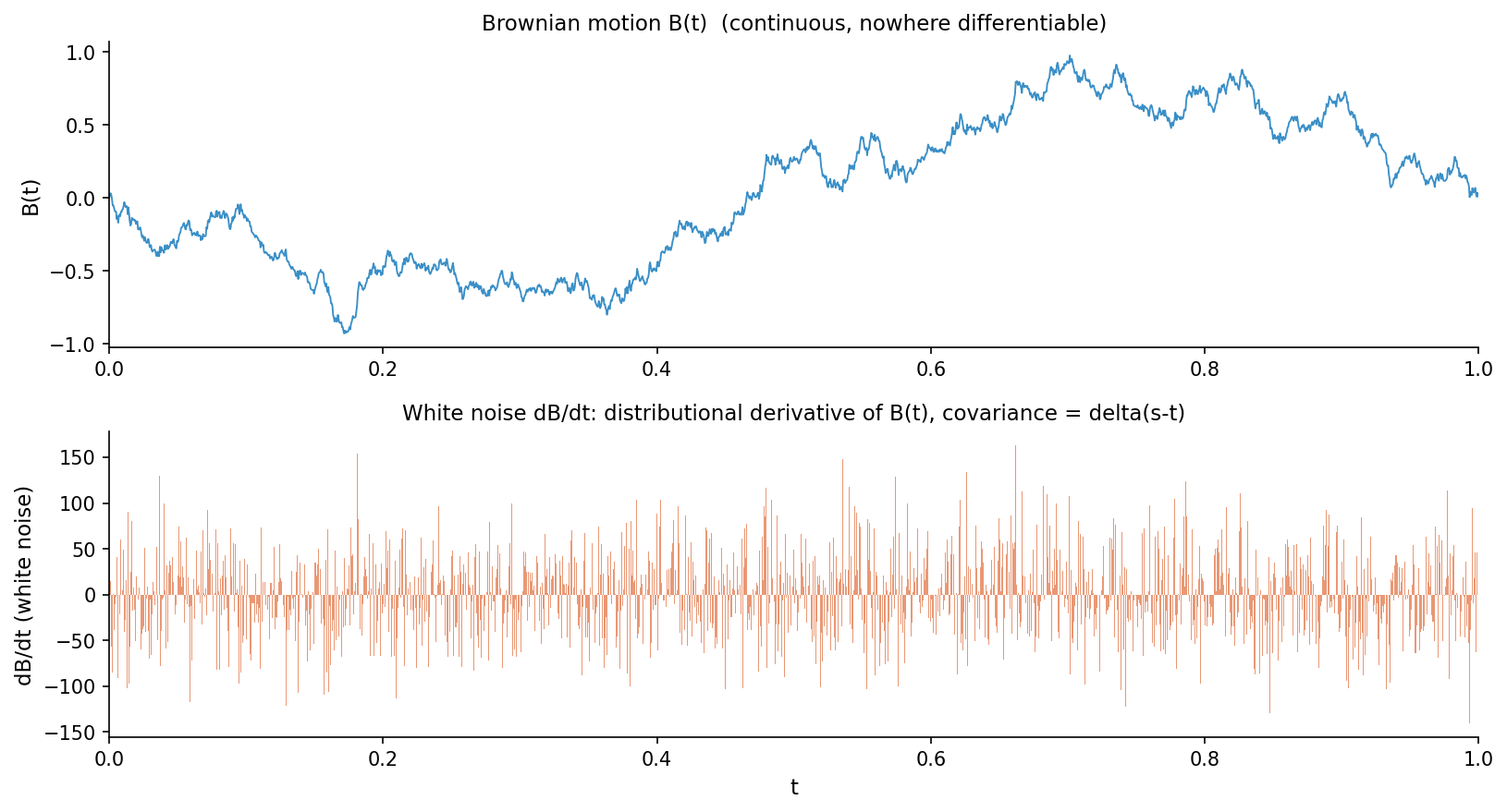
White noise as derivative of Brownian motion

চিত্র ৭: উপরে: Brownian motion \(B_t\) (continuous)। নিচে: white noise \(dB/dt\) — discrete increments দিয়ে approximation। প্রতিটা মুহূর্তে স্বাধীন, covariance = \(\delta(s-t)\)।

White Noise-এর নাম কেন?

White noise-এর Fourier transform-এ সব frequency-র contribution সমান — ঠিক white light-এ সব রঙ আছে। তাই নাম "white" noise।

৬. সাধারণ ভুল (Common Mistakes)¶

৪টি সাধারণ ভুল

১. Brownian path মসৃণ মনে করা। \(B_t\) continuous, কিন্তু differentiable নয়। \(dB_t / dt\) ordinary derivative হিসেবে exist করে না।

২. Variance এবং Standard Deviation গুলিয়ে ফেলা। \(\text{Var}(B_t) = t\), কিন্তু \(\text{std}(B_t) = \sqrt{t}\)। Spread \(\sqrt{t}\)-এ বাড়ে, \(t\)-এ নয়।

৩. Independent increment মানে independent values ভাবা। \(B_s\) এবং \(B_t\) (s < t) স্বাধীন নয় — \(\text{Cov}(B_s, B_t) = \min(s,t) \neq 0\)। Increments স্বাধীন, values নয়।

৪. Wiener measure = Lebesgue measure মনে করা। Wiener measure একটি infinite-dimensional space \(C[0,\infty)\)-এ থাকে; Lebesgue measure \(\mathbb{R}^n\)-এ। এদের সরাসরি তুলনা হয় না।

৭. এক্সারসাইজ (Exercises)¶

সমস্যা ১. দেখাও যে \(\text{Var}(B_t - B_s) = t - s\) যখন \(0 \leq s \leq t\)।

সমস্যা ২. \(c > 0\)-এর জন্য, \(\tilde{B}_t := c^{-1/2} B_{ct}\) define করো। দেখাও \(\{\tilde{B}_t\}\) একটি standard Brownian motion।

সমস্যা ৩. \(M_t := B_t^2 - t\) define করো। দেখাও \(\mathbb{E}[M_t] = 0\) এবং \(\mathbb{E}[M_t^2] = 2t^2\)।

সমস্যা ৪. Heat kernel \(p(x,y;t)\) verify করো: \(\int_\mathbb{R} p(x,y;t)\, dy = 1\) এবং \(\int_\mathbb{R} p(x,y;s) p(y,z;t)\, dy = p(x,z;\,s+t)\)।

সমস্যা ৫. White noise \(\dot{B}\) এর variance \(\text{Var}(\langle \dot{B}, \phi \rangle) = \int_0^\infty \phi(t)^2\, dt\) হওয়ার calculation-টি সম্পূর্ণ করো (integration by parts ব্যবহার করো)।

সমস্যা ৬. Covariance function \(\text{Cov}(B_s, B_t) = \min(s,t)\) থেকে দেখাও যে \(B_s\) এবং \(B_t - B_s\) (s < t) uncorrelated — এবং Gaussian হওয়ার কারণে তারা actually স্বাধীন।

৮. সমাধান (ব্যাখ্যাসহ)¶

১-নং সমাধান দেখাও

সমস্যা ১: \(\text{Var}(B_t - B_s) = t - s\)।

সংজ্ঞা থেকে: \(B_t - B_s \sim N(0, t-s)\)।

একটি \(N(0, \sigma^2)\) random variable-এর variance হলো \(\sigma^2\)।

এখানে \(\sigma^2 = t - s\)। তাই \(\text{Var}(B_t - B_s) = t - s\)। \(\square\)

২-নং সমাধান দেখাও

সমস্যা ২: \(\tilde{B}_t = c^{-1/2} B_{ct}\) is standard BM।

চেক করি চারটি শর্ত:

(a) \(\tilde{B}_0 = c^{-1/2} B_0 = 0\)। ✓

(b) \(\tilde{B}_t - \tilde{B}_s = c^{-1/2}(B_{ct} - B_{cs})\)।

\(B_{ct} - B_{cs} \sim N(0, ct - cs) = N(0, c(t-s))\)।

তাই \(c^{-1/2}(B_{ct} - B_{cs}) \sim N(0, c^{-1} \cdot c(t-s)) = N(0, t-s)\)। ✓

(c) \(B_{ct}\)-এর independent increments থেকে \(\tilde{B}\)-এরও independent increments আসে। ✓

(d) \(B_{ct}\) continuous, তাই \(c^{-1/2} B_{ct}\)-ও continuous। ✓

সব শর্ত পূরণ, তাই \(\tilde{B}\) একটি standard BM। \(\square\)

৩-নং সমাধান দেখাও

সমস্যা ৩: \(M_t = B_t^2 - t\)।

\(\mathbb{E}[B_t^2] = \text{Var}(B_t) + (\mathbb{E}[B_t])^2 = t + 0 = t\)।

তাই \(\mathbb{E}[M_t] = \mathbb{E}[B_t^2] - t = t - t = 0\)। ✓

\(M_t^2 = B_t^4 - 2tB_t^2 + t^2\)।

\(B_t \sim N(0,t)\) হলে \(B_t = \sqrt{t}\,Z\) যেখানে \(Z \sim N(0,1)\)।

\(\mathbb{E}[Z^4] = 3\) (Gaussian-এর fourth moment)।

তাই \(\mathbb{E}[B_t^4] = t^2 \cdot 3 = 3t^2\)।

\[\mathbb{E}[M_t^2] = 3t^2 - 2t \cdot t + t^2 = 3t^2 - 2t^2 + t^2 = 2t^2. \quad \square\]

৪-নং সমাধান দেখাও

সমস্যা ৪: Heat kernel properties।

Normalization: \(p(x,y;t) = \frac{1}{\sqrt{2\pi t}} e^{-(x-y)^2/(2t)}\)।

\(\int_\mathbb{R} p(x,y;t)\, dy = \int_\mathbb{R} \frac{1}{\sqrt{2\pi t}} e^{-(x-y)^2/(2t)}\, dy\)।

Substitution \(u = (y-x)/\sqrt{t}\): \(= \int_\mathbb{R} \frac{1}{\sqrt{2\pi}} e^{-u^2/2}\, du = 1\)। ✓

Semi-group property: Fourier transform-এ,

\(\hat{p}(\xi; t) = e^{-t\xi^2/2}\)।

Convolution in \(y\) → product in Fourier: \(e^{-s\xi^2/2} \cdot e^{-t\xi^2/2} = e^{-(s+t)\xi^2/2} = \hat{p}(\xi;\, s+t)\)। \(\square\)

৫-নং সমাধান দেখাও

সমস্যা ৫: \(\text{Var}(\langle \dot{B}, \phi \rangle) = \int_0^\infty \phi(t)^2\, dt\)।

\(\langle \dot{B}, \phi \rangle = -\langle B, \dot{\phi} \rangle\), তাই variance:

\[\text{Var} = \int_0^\infty \int_0^\infty \min(s,t)\, \dot{\phi}(s)\, \dot{\phi}(t)\; ds\, dt\]

\[= 2\int_0^\infty \int_0^t s\, \dot{\phi}(s)\, \dot{\phi}(t)\; ds\, dt\]

Inner integral (integration by parts in \(s\)):

\[\int_0^t s\, \dot{\phi}(s)\, ds = \bigl[s\,\phi(s)\bigr]_0^t - \int_0^t \phi(s)\, ds = t\phi(t) - \int_0^t \phi(s)\, ds\]

Now integrate over \(t\) (by parts again):

\[2\int_0^\infty t\phi(t)\dot{\phi}(t)\, dt = \bigl[t\phi(t)^2\bigr]_0^\infty - \int_0^\infty \phi(t)^2\, dt - \int_0^\infty t\phi(t)\dot{\phi}(t)\, dt\]

(boundary terms vanish for \(\phi \in \mathcal{S}\)), giving:

\[2\int_0^\infty t\phi(t)\dot{\phi}(t)\, dt = -\int_0^\infty \phi(t)^2\, dt\]

The second part: \(-2\int_0^\infty \bigl(\int_0^t \phi(s)\, ds\bigr)\dot{\phi}(t)\, dt = 2\int_0^\infty \phi(t)^2\, dt\)।

Combining: \(-\int_0^\infty \phi^2\, dt + 2\int_0^\infty \phi^2\, dt = \int_0^\infty \phi(t)^2\, dt\)। \(\square\)

৬-নং সমাধান দেখাও

সমস্যা ৬: \(B_s\) এবং \(B_t - B_s\) স্বাধীন (\(s < t\))।

Covariance:

\[\text{Cov}(B_s,\; B_t - B_s) = \mathbb{E}[B_s(B_t - B_s)]\]

\[= \mathbb{E}[B_s B_t] - \mathbb{E}[B_s^2] = \min(s,t) - s = s - s = 0\]

তাই uncorrelated। \((B_s, B_t - B_s)\) jointly Gaussian (কারণ Gaussian increments সংজ্ঞার অংশ)।

Jointly Gaussian + uncorrelated \(\Rightarrow\) independent। \(\square\)

৯. সারসংক্ষেপ ও Checklist¶

[ ] Brownian motion-এর চারটি defining property জানি: \(B_0=0\), continuous paths, independent Gaussian increments \(B_t - B_s \sim N(0, t-s)\)
[ ] Wiener measure হলো \(C[0,\infty)\)-এর উপর একটি probability measure যা Brownian motion কে rigorous করে
[ ] Heat kernel \(p(x,y;t)\)-এর semi-group property বুঝি: \(p(\cdot;\,s) * p(\cdot;\,t) = p(\cdot;\,s+t)\)
[ ] Brownian paths continuous কিন্তু nowhere differentiable — zoom করলে একই jagged structure
[ ] Spread \(\sqrt{t}\)-এ বাড়ে; scaling: \(c^{-1/2}B_{ct} \overset{d}{=} B_t\)
[ ] Covariance \(\text{Cov}(B_s, B_t) = \min(s,t)\)
[ ] White noise \(\dot{B}\) হলো \(B_t\)-এর distributional derivative; covariance function = \(\delta(s-t)\)

➡️ পরের অধ্যায়: 7.4 — Haar Measure — locally compact group-এর উপর translation-invariant measure; existence ও uniqueness (up to scale); উদাহরণ \(\mathbb{R}\), \(\mathbb{Z}\), \(S^1\), matrix groups।